Math

Distance and Similarity Metrics

Several defensible ways to measure how alike two things are, which disagree with each other — so picking one is a modelling decision, not a formatting choice.

Cosine and Euclidean can disagree completely: two vectors pointing the same way but very different lengths are identical by angle and far apart by distance

Why Does This Exist?

Every vector database setup asks you to pick a metric from a dropdown, offers no explanation, and then never mentions it again. That dropdown decides your search quality, and the three options do not merely differ in scale — they can rank the same candidates in opposite orders.

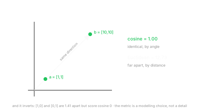
The demonstration is in the diagram. Take $a = [1,1]$ and $b = [10,10]$ : cosine similarity says they are identical, and Euclidean distance says they are 12.7 apart. Now take $[1,0]$ and $[0,1]$ : Euclidean says 1.41, closer than the first pair, while cosine says 0 — completely unrelated. The two metrics have inverted the ranking.

This is the page behind the most common retrieval bug there is, and behind a subtler one: k-nearest neighbours and k-means both silently assume Euclidean, so feeding them unscaled features means the largest-range feature decides every neighbour.

Think of It Like This

Two ways to say two people are similar

Two people describe how much they like ten films, scoring each out of ten.

One is generous and rates everything 8 to 10. The other is harsh and rates the same films 2 to 4. Ask "are their tastes similar?" and you get two defensible answers.

By distance, they could not be further apart — every single score differs by six points. By direction, they are nearly identical: both rank the same films highest and lowest, and one is simply the other shifted down. Their pattern of preferences agrees completely.

Which answer is right depends on what you are building. A recommender wants direction, because it cares about relative preference and not about whether someone is a generous rater. A quality-control system wants distance, because the absolute values are the thing being checked.

That is the whole content of metric choice, and it is why the dropdown matters. You are declaring what "similar" means for your problem.

How It Actually Works

Four measures cover nearly all practical use.

Euclidean (L2) distance — straight-line separation:

d(a,b) = \lVert a - b \rVert_2 = \sqrt{\textstyle\sum_i (a_i - b_i)^2}

Sensitive to magnitude, and the default assumption of k-NN, k-means, and most clustering.

Cosine similarity — the angle only:

\cos\theta = \frac{a \cdot b}{\lVert a\rVert_2\,\lVert b\rVert_2}

Bounded in $[-1, 1]$ , completely blind to length. The default for embeddings. Note "cosine distance" usually means $1 - \cos\theta$ , which is not a true metric — it violates the triangle inequality — so it cannot be used in algorithms that require one.

Dot product — $a \cdot b$ , unnormalised. Mixes direction and both magnitudes, which is the trap: a long irrelevant vector beats a short relevant one. Fast, and correct only when your vectors are already unit length.

Manhattan (L1) distance — $\sum_i |a_i - b_i|$ . Less sensitive to a single large discrepancy than Euclidean, since it does not square. Sometimes preferred in high dimensions for that reason.

The identity that resolves most of it

For unit-length vectors, Euclidean distance and cosine similarity are the same ranking:

\lVert a - b \rVert_2^2 = 2 - 2\cos\theta

In plain words: once both vectors have length 1, squared distance is a decreasing function of cosine similarity, so sorting by one sorts by the other. The metrics stop disagreeing.

Expand $\lVert a - b\rVert^2 = a \cdot a - 2 a \cdot b + b \cdot b = 1 - 2\cos\theta + 1$ to see it. This is why normalising at ingestion is such a clean move: normalise once, then the cheap dot product is cosine similarity, and Euclidean agrees with both. The dropdown genuinely stops mattering.

Choosing

Embeddings from a neural model — cosine, or dot product on pre-normalised vectors. Magnitude is a training artifact, not meaning.
Physical measurements in real units — Euclidean, after standardising features so no unit dominates.
Sparse count vectors (TF-IDF, bag of words) — cosine. Document length would otherwise dominate.
Recommender inner products — dot product deliberately, because in matrix factorisation the magnitude encodes popularity and you may want that.
Sets rather than vectors — Jaccard, the size of the intersection over the union. Different family, and the right answer for tags or shingles.

High dimensions change the picture

In very high dimensions distances concentrate: the ratio between the nearest and farthest neighbour of a random point approaches 1, so "nearest" becomes weakly meaningful. This is one face of the curse of dimensionality, and it hits Euclidean harder than cosine.

Real embeddings are less affected than random vectors, because they occupy a low-dimensional manifold rather than filling the space. But the effect is why cosine dominates for high-dimensional embeddings, and why approximate nearest-neighbour indexes can afford to be approximate — the distances they are approximating are close together anyway.

Worked example

Take $a = [1, 1]$ and $b = [10, 10]$ , so $b = 10a$ — exactly the same direction.

Norms: $\lVert a \rVert = \sqrt{2} \approx 1.414$ and $\lVert b \rVert = \sqrt{200} \approx 14.142$ . Dot product: $1{\cdot}10 + 1{\cdot}10 = 20$ .

\cos\theta = \frac{20}{1.414 \times 14.142} = \frac{20}{20} = 1

Perfect similarity — correct, since they are parallel. But the Euclidean distance:

d = \sqrt{(1-10)^2 + (1-10)^2} = \sqrt{81 + 81} = 9\sqrt{2} \approx 12.73

Very far apart. Same pair, opposite verdicts.

Now invert it with $c = [1, 0]$ and $d = [0, 1]$ . Euclidean distance is $\sqrt{1 + 1} \approx 1.414$ — much closer than the first pair. Cosine similarity is $0/(1 \times 1) = 0$ — orthogonal, no similarity at all.

So by Euclidean, $(c,d)$ at 1.41 is far closer than $(a,b)$ at 12.73. By cosine, $(a,b)$ at 1.0 beats $(c,d)$ at 0.0. The ranking has completely reversed, from four vectors and no ambiguity.

Finally, normalise and watch the disagreement vanish. $\hat a = \hat b = [0.707, 0.707]$ , so their distance becomes 0 and their cosine stays 1. Both metrics now agree they are identical.

Show Me the Code

1import numpy as np2
3
4def cosine(u: np.ndarray, v: np.ndarray) -> float:5    return float(u @ v / (np.linalg.norm(u) * np.linalg.norm(v)))6
7
8a, b = np.array([1.0, 1.0]), np.array([10.0, 10.0])   # same direction9c, d = np.array([1.0, 0.0]), np.array([0.0, 1.0])     # orthogonal10
11print(round(cosine(a, b), 4), round(float(np.linalg.norm(a - b)), 4))  # -> 1.0 12.727912print(round(cosine(c, d), 4), round(float(np.linalg.norm(c - d)), 4))  # -> 0.0 1.414213
14# Normalising makes the two metrics agree: ||a-b||^2 == 2 - 2*cos.15u, v = a / np.linalg.norm(a), b / np.linalg.norm(b)16print(round(float(np.linalg.norm(u - v) ** 2), 10),17      round(2 - 2 * cosine(u, v), 10))                # -> 0.0 0.018
19# Unscaled features let the widest-range column decide every neighbour.20X = np.array([[1.0, 1000.0], [2.0, 1000.0], [1.0, 2000.0]])   # (3, 2)21print(round(float(np.linalg.norm(X[0] - X[1])), 3),22      round(float(np.linalg.norm(X[0] - X[2])), 3))    # -> 1.0 1000.0

Every number matches the hand calculation. The last block is the k-NN failure: rows 0 and 1 differ by 1 in feature one, rows 0 and 2 by 1000 in feature two, and Euclidean distance treats the second as a thousand times more important purely because of units.

Watch Out For

Using Euclidean distance on unstandardised features

Euclidean distance sums squared differences across features, so a feature with a wide numeric range contributes far more than a narrow one — regardless of how informative either is.

Put income in dollars (range ~ $10^5$ ) alongside age in years (range ~ $10^2$ ) and the squared income difference dwarfs everything. Your k-NN classifier is effectively a one-feature model using income, and your k-means clusters are income bands. Nothing errors, accuracy is mediocre-but-plausible, and people go looking for better values of $k$ .

The fix is standardisation before any distance-based method: subtract the mean and divide by the standard deviation per feature, so each contributes comparably. StandardScaler inside a pipeline, fitted on training data only — fitting on the full dataset leaks test statistics into training.

Two refinements worth knowing. If features are correlated, even standardised Euclidean over-counts the shared information, and Mahalanobis distance — which divides by the covariance rather than just the variances — is the principled answer. And if a feature genuinely deserves more weight, scale it deliberately and write down why, rather than letting its unit decide.

Assuming your index's metric matches your training objective

The most expensive version of this bug is a mismatch between how embeddings were trained and how they are searched.

Models trained with a contrastive objective on cosine similarity produce vectors whose angles are meaningful and whose magnitudes are not. Search that index with inner product on unnormalised vectors and you have changed the objective: results are now ranked partly by magnitude, which correlates with document length and token frequency rather than relevance. Quality drops a few points, no test fails, and the cause is a dropdown chosen weeks earlier.

It also cuts the other way. Matrix-factorisation recommenders trained with an inner-product objective deliberately encode popularity in the magnitude. Normalise those vectors and you throw away real signal, flattening the popularity prior the model learned.

Two habits close it. Write down the training objective's metric next to the index configuration, and make them match. And assert the invariant — if the index expects unit vectors, check np.linalg.norm(v) is 1.0 within tolerance at write time. That single assertion catches the whole class of failure, and almost nobody writes it.

The Quick Version

Euclidean is straight-line distance and is magnitude-sensitive. Cosine is angle only, bounded in $[-1,1]$ .
Raw dot product mixes direction with both magnitudes, so long vectors win. Correct only on pre-normalised vectors.
The metrics can rank pairs in opposite orders: $[1,1]$ vs $[10,10]$ is cosine 1.0 and distance 12.73.
For unit vectors, $\lVert a-b\rVert^2 = 2 - 2\cos\theta$ , so both give the same ranking. Normalise once at ingestion and the choice stops mattering.
"Cosine distance" $1 - \cos\theta$ is not a true metric — it fails the triangle inequality.
Embeddings → cosine. Physical units → standardised Euclidean. Sparse counts → cosine. Sets → Jaccard.
In high dimensions distances concentrate, so "nearest" weakens. Cosine holds up better than Euclidean.
Standardise features before any distance-based method, or the widest-range feature decides every neighbour.
Match your index metric to your training objective, and assert the unit-norm invariant at write time.