Math

Integration and Area Under a Curve

Adding up infinitely many infinitely thin slices to get a total — and the surprising fact that doing so is just differentiation run backwards.

An integral is the area trapped under a curve, approximated by rectangles that get thinner until the staircase becomes the curve itself

Why Does This Exist?

Every continuous probability distribution you use is defined by an integral. The Gaussian's bell curve means nothing until you know that the area under it between two points is the probability of landing there — and that its total area is exactly 1. Ask what "AUC" stands for in ROC-AUC and the answer is area under the curve, which is an integral. The intractable term that makes variational autoencoders hard is an integral. Expected values over continuous variables are integrals.

So this page exists because the band cannot honestly talk about continuous probability without it. Probability distributions already tells you a density "integrates to 1" — this is the page that makes that sentence mean something.

There is a second, more practical reason. Most integrals you meet in ML have no closed-form answer, and knowing that is the actual skill. Recognising an integral, understanding why it resists solving, and reaching for sampling instead is what separates someone who can read a VAE paper from someone who cannot.

Think of It Like This

A car with a broken odometer

Your odometer is dead but your speedometer works. You want to know how far you have travelled.

Drive at a steady 60 km/h for two hours and it is easy: distance is speed times time, 120 km. That is the area of a rectangle two units wide and sixty tall.

Now the speed varies constantly. The trick still works if you cheat a little — glance at the speedometer every minute and pretend the speed was constant for that minute. Sixty small rectangles, added up, and you get a decent estimate. Check every second instead and you get a better one. The narrower each slice, the less the pretence costs you.

An integral is what that estimate converges to as the slices become infinitely thin. And the punchline of the whole subject is that distance and speed are already related: speed is the derivative of distance. So integrating the speedometer must recover the odometer, which means integration undoes differentiation. That is not a coincidence, it is the fundamental theorem.

How It Actually Works

Two ideas that turn out to be the same idea.

Integration as accumulated area

Take a function $f$ over an interval from $a$ to $b$ . Chop the interval into $n$ slices of width $\Delta x$ , and on each slice approximate $f$ by a constant, giving a rectangle. Adding the rectangles gives a Riemann sum:

\sum_{i=1}^{n} f(x_i)\, \Delta x

In plain words: height times width, totalled over every slice. As the slices get thinner the sum converges, and the limit is the definite integral:

\int_a^b f(x)\, dx

The notation is a picture of the sum. The $\int$ is an elongated S for "sum", $f(x)$ is the height, and $dx$ is the infinitesimally thin width. Two properties follow immediately and both get used constantly: the integral is additive over intervals, so $\int_a^c = \int_a^b + \int_b^c$ , and area below the axis counts as negative.

The antiderivative, and the theorem that connects them

An antiderivative $F$ of $f$ is any function whose derivative is $f$ . Since $\frac{d}{dx}\frac{x^3}{3} = x^2$ , the function $x^3/3$ is an antiderivative of $x^2$ .

The fundamental theorem of calculus says the area is just the change in the antiderivative across the interval:

\int_a^b f(x)\, dx = F(b) - F(a)

In plain words: to find an area, find any function whose slope is your curve, and subtract its values at the two endpoints. This is remarkable — a limit of infinitely many rectangles collapses to one subtraction. It is also why the two halves of calculus are one subject rather than two.

Antiderivatives are only unique up to a constant, since a constant differentiates to zero. That constant cancels in the subtraction, so it never affects a definite integral.

The rules you actually need

For ML, three suffice. Powers: $\int x^n dx = \frac{x^{n+1}}{n+1} + C$ for $n \neq -1$ . The exponential: $\int e^x dx = e^x + C$ , which is the one that makes Gaussians tractable. And the reciprocal: $\int \frac{1}{x} dx = \ln|x| + C$ , which is where logarithms come from.

For multiple variables you integrate one at a time, holding the others fixed — the same "freeze everything else" move that makes a partial derivative work. A double integral over a region is just an integral of an integral.

The honest part: most integrals cannot be solved

Differentiation is mechanical. Given any expression built from standard functions, the chain and product rules crank out its derivative.

Integration is not. Many perfectly ordinary functions have no antiderivative expressible in elementary terms, and the most famous example is $e^{-x^2}$ — the Gaussian. There is no formula for the area under a bell curve between two arbitrary points. This is not a gap in anyone's knowledge; it is provably impossible, which is why statistics tables existed and why scipy.stats.norm.cdf is a numerical routine rather than an algebraic one.

That fact shapes practical ML more than any integration technique:

Numerical quadrature — do the Riemann sum with clever slice placement. Excellent in one or two dimensions, useless in a thousand.
Monte Carlo — sample points at random and average. Its error shrinks like $1/\sqrt{N}$ regardless of dimension, which is why it is the only viable option in high dimensions and why sampling appears everywhere in Bayesian ML.

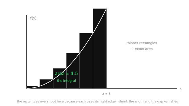
Look again at the diagram: the Riemann rectangles are the picture of a Monte Carlo estimate, except Monte Carlo places its slices randomly instead of on a grid.

Worked example

Integrate $f(x) = x^2$ from 0 to 3.

An antiderivative is $F(x) = x^3/3$ . Check by differentiating: $\frac{d}{dx}\frac{x^3}{3} = x^2$ . Then:

\int_0^3 x^2\, dx = \frac{3^3}{3} - \frac{0^3}{3} = 9 - 0 = 9

In plain words: the area under the parabola between 0 and 3 is exactly 9 square units.

Now check it against a Riemann sum with six slices of width 0.5, using each slice's right edge. Heights are $f(0.5) = 0.25$ , $f(1) = 1$ , $f(1.5) = 2.25$ , $f(2) = 4$ , $f(2.5) = 6.25$ , $f(3) = 9$ . Their total is 22.75, times the width 0.5 gives 11.375.

That overshoots 9 by a lot, and the reason is visible in the diagram: on a rising curve, the right edge is the tallest point in each slice, so every rectangle pokes above the curve. Halve the width to 0.25 and the estimate falls to about 10.16; at width 0.01 it is 9.07. Converging, but slowly — the error shrinks in proportion to the slice width, which is why nobody uses plain right-endpoint sums for real work.

The diagram's shaded area corresponds to the same $f(x) = x^2/2$ family and shows 4.5, which is exactly half of 9 — the same integral with the function halved.

Show Me the Code

1import numpy as np2
3
4def riemann_right(f, a: float, b: float, n: int) -> float:5    dx = (b - a) / n6    x = a + dx * np.arange(1, n + 1)   # right edge of each slice, shape (n,)7    return float(np.sum(f(x) * dx))8
9
10f = lambda x: x**211print(round(riemann_right(f, 0, 3, 6), 4))       # -> 11.375   coarse, overshoots12print(round(riemann_right(f, 0, 3, 300), 4))     # -> 9.045113print(round(riemann_right(f, 0, 3, 30_000), 4))  # -> 9.0005   -> the exact 914
15# Monte Carlo: average the height at random points, times the width.16rng = np.random.default_rng(0)17xs = rng.uniform(0, 3, size=100_000)18print(round(float(np.mean(f(xs)) * 3), 3))        # -> approx 9.0, no grid needed

The exact answer is 9, and both routes approach it. The contrast is the lesson: the Riemann sum needs its slices placed on a grid, which becomes hopeless in high dimensions, while the Monte Carlo estimate only needs the ability to sample.

Watch Out For

Shrinking the step size past the point where it helps

Numerical integration has the same U-shaped error curve as numerical differentiation, and for the same reason.

Halving the slice width halves the truncation error, so finer looks strictly better. But it also doubles the number of terms you add, and every floating-point addition rounds. Summing 10 million values, each carrying a rounding error, accumulates error that grows with the count — while each term shrinks toward the point where adding it to a large running total changes nothing at all. Past a certain $n$ , the accumulated round-off overtakes the truncation you were trying to remove, and the answer gets worse.

The practical defence is not a smaller step. It is a better rule and a better sum: the trapezoid rule and Simpson's rule converge far faster for the same number of evaluations, and math.fsum or pairwise summation keeps the accumulation error from growing linearly. scipy.integrate.quad does both and reports an error estimate, which is the number to check rather than assume.

Reaching for quadrature in high dimensions

Grid-based integration dies exponentially with dimension, and the arithmetic is worth doing once so you never try it.

Ten slices per axis is a crude grid. In 2 dimensions that is 100 evaluations — fine. In 10 dimensions it is $10^{10}$ , which is already a serious compute job. In 100 dimensions it is $10^{100}$ , more evaluations than there are atoms in the observable universe. A latent space of 100 dimensions is small by modern standards.

This is the curse of dimensionality in its most concrete form, and it is the reason Bayesian ML is built on sampling rather than on quadrature. Monte Carlo error scales as $1/\sqrt{N}$ with no dimension term — a thousand samples give roughly the same accuracy in 100 dimensions as in 2. It converges slowly, needing 100 times the samples for 10 times the accuracy, but it converges at all, which quadrature does not.

So when you meet an integral over a latent space or a posterior, the question is never "which integration technique" — it is "can I sample from this, and if not, can I reshape it into something I can sample from". That reshaping is what the reparameterisation trick and importance sampling do.

The Quick Version

A definite integral is the limit of a Riemann sum: heights times widths, with the widths going to zero.
It is signed — area below the axis subtracts — and additive over adjacent intervals.
An antiderivative is a function whose derivative is your function.
The fundamental theorem: $\int_a^b f = F(b) - F(a)$ . A limit of infinite rectangles collapses to one subtraction.
Integration undoes differentiation. That is why the two halves of calculus are one subject.
Three rules cover most ML needs: powers, $e^x$ , and $1/x$ giving $\ln|x|$ .
Most integrals have no closed form. $e^{-x^2}$ , the Gaussian, provably does not — which is why norm.cdf is numerical.
Grid quadrature costs $k^d$ and is unusable past a few dimensions. Monte Carlo error is $1/\sqrt{N}$ regardless of dimension.