Maximum Likelihood Estimation

Why Does This Exist?

Training a neural network is maximum likelihood estimation. Not an analogy — the same procedure, with a different function being optimised.

This is the page that turns a pile of separate-looking loss functions into one idea. Cross-entropy for classification, mean squared error for regression, the objective behind language model pretraining: all three are the negative log-likelihood of an assumed distribution, and all three are minimised by the same reasoning. Once you have this, you stop memorising which loss goes with which task and start deriving it.

The practical value is that it tells you what to do when your problem does not fit a standard loss. Predicting counts, or a value that must stay positive, or something with heavy tails? There is no lookup table entry for those — but there is a procedure. Write down the distribution you believe your data came from, take its negative log-likelihood, and you have your loss function. That is the whole method, and it is why L2 regularisation turns out to be a Gaussian prior rather than a trick someone found.

Think of It Like This

How It Actually Works

Given observed data $D$ and a model with parameters $\theta$, the likelihood is the probability of the data under those parameters:

In plain words: how probable is what I actually saw, if these parameter values were the truth? Read the direction carefully, because it is the part people get backwards. The data is fixed and known; $\theta$ is what varies. The likelihood is a function of the parameters, not of the data.

For $n$ independent observations the joint probability is a product:

The estimate $\hat{\theta}$ is whichever $\theta$ makes that largest.

Take the log, then negate

That product is unusable as written. A thousand probabilities each around 0.1 multiply to $10^{-1000}$, which underflows to exactly zero in any float type — so the objective becomes flat zero everywhere and there is nothing to optimise.

Taking the logarithm turns the product into a sum:

In plain words: add up the log-probability of every observation instead of multiplying the probabilities. This is safe because $\log$ is strictly increasing, so it never moves the location of the maximum — only its value. Sums of a thousand numbers around $-2.3$ are perfectly well-behaved.

Then negate, because optimisers minimise:

That is the negative log-likelihood, and it is your loss function. Every step here was mechanical — none of it involved choosing a loss.

Where the standard losses come from

Now run the procedure on each of the three common assumptions:

• Categorical (multi-class classification). $P(y_i \mid x_i, \theta)$ is the softmax probability of the true class, so the negative log-likelihood is $-\sum \log \hat{y}_{i,\text{true}}$ — exactly cross-entropy loss.
• Bernoulli (binary classification). The negative log-likelihood is $-\sum [y \log \hat{y} + (1-y)\log(1-\hat{y})]$ — binary cross-entropy, term for term.
• Gaussian with fixed variance (regression). The Gaussian density has $e^{-(y-\hat{y})^2 / 2\sigma^2}$ in it, so its log is $-(y - \hat{y})^2 / 2\sigma^2$ plus a constant. Negate and the constants drop out under optimisation, leaving $\sum (y - \hat{y})^2$ — mean squared error.

That last one is worth pausing on. MSE squares its errors because the Gaussian has a square in its exponent. Not for convenience, not because it is differentiable — because of the distribution you assumed. Swap in a Laplace distribution and the same procedure gives you mean absolute error, which is more tolerant of outliers precisely because the Laplace has fatter tails.

Adding a prior gives you regularisation

Maximum likelihood asks only which $\theta$ best explains the data, which means it will happily choose extreme parameter values if they fit slightly better. That is overfitting, stated in probabilistic terms.

Bayes' theorem offers the fix. Instead of maximising $P(D \mid \theta)$, maximise $P(\theta \mid D) \propto P(D \mid \theta) P(\theta)$, where $P(\theta)$ encodes what you believed about the parameters beforehand. This is MAP estimation, and taking logs turns the product into a sum:

In plain words: your usual loss, plus a penalty for parameter values you considered implausible to begin with. Assume a zero-centred Gaussian prior on the weights and $-\log P(\theta)$ works out to $\lambda \lVert \theta \rVert_2^2$ — L2 regularisation is a Gaussian prior. Assume a Laplace prior instead and you get $\lambda \lVert \theta \rVert_1$, which is L1, and its sparsity is the Laplace distribution's spike at zero showing through. See norms for the geometry of why that spike produces exact zeros.

Worked example

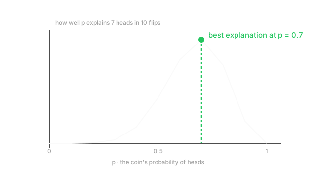
Flip a coin ten times and get seven heads. What is the coin's probability of heads?

With $p$ as the unknown, each head contributes a factor of $p$ and each tail a factor of $(1-p)$:

In plain words: how likely is seven heads and three tails, if the coin's true bias were $p$? That is the curve in the diagram above. Take the log:

The maximum is where the derivative is zero:

Multiply through by $p(1-p)$ to get $7(1-p) = 3p$, so $7 = 10p$ and:

The answer is the observed proportion, which is reassuring — but notice it was derived, not assumed. That same derivation on a Gaussian returns the sample mean, and on a categorical returns the observed class frequencies. Maximum likelihood recovers the obvious estimator when the obvious estimator is right, and tells you what to do when it is not.

Worth seeing the failure case too: ten heads out of ten gives $\hat{p} = 1.0$, meaning the model declares tails impossible on ten observations. That is maximum likelihood being overconfident with small data, and it is exactly what a prior fixes.

Show Me the Code

1import numpy as np2
3
4def neg_log_likelihood(p: float, heads: int, tails: int) -> float:5    # Sum of log-probabilities, never a product — the product underflows.6    return -(heads * np.log(p) + tails * np.log(1 - p))7
8
9grid = np.linspace(0.01, 0.99, 99)                       # candidate values of p10nll = np.array([neg_log_likelihood(p, 7, 3) for p in grid])11print(round(float(grid[nll.argmin()]), 2))               # -> 0.7   matches 7/1012
13# Why the log is not optional: 1000 observations as a raw product.14print(np.prod(np.full(1000, 0.1)))                       # -> 0.0    underflowed15print(np.sum(np.log(np.full(1000, 0.1))))                # -> -2302.58...  fine

The grid search lands on 0.70, matching the calculus. The last two lines are the reason every implementation works in log space.

Watch Out For

The Quick Version

• Maximum likelihood picks the parameters under which the observed data is least surprising.
• The likelihood $P(D \mid \theta)$ is a function of the parameters; the data is fixed.
• Products of many probabilities underflow, so always work with the log — it is monotone, so the maximum does not move.
• Negate the log-likelihood and you have your loss function. That is where losses come from.
• Categorical assumption gives cross-entropy. Bernoulli gives binary cross-entropy. Gaussian gives MSE.
• MSE squares errors because the Gaussian squares in its exponent. Laplace instead gives mean absolute error.
• Multiplying in a prior gives MAP: L2 regularisation is a Gaussian prior, L1 is a Laplace prior.
• $P(D \mid \theta)$ is not $P(\theta \mid D)$. A likelihood is not a belief about the parameters.
• MLE assigns probability zero to anything unseen, which becomes $-\infty$ in log space. Smoothing is a prior.

What to Read Next

• Cross-Entropy is the loss this procedure produces for classification.
• Probability Distributions is the assumption you have to make before the procedure can run.
• Gradients is how the resulting loss is actually minimised.
• Norms explains why a Laplace prior yields exact zeros and a Gaussian one does not.
• Definitions worth a look: Likelihood, Log-Likelihood, Bayes' Theorem, and Normal Distribution.
• Related interview question: What is maximum likelihood estimation?