Math

Cross-Entropy

The price you pay for being confidently wrong: it reads off the probability your model gave the correct answer and charges you the negative logarithm of it.

Why Does This Exist?

Classification needs a loss that punishes confident mistakes far harder than hesitant ones, and accuracy cannot do it. A model that says 51% for the right class and one that says 99% both count as correct, and both score identically. There is no gradient to follow, so there is nothing to train on.

Cross-entropy fixes exactly this. A prediction of 0.99 on the right answer costs 0.01. A prediction of 0.01 on it costs 4.6 — over four hundred times as much. Being confidently wrong is expensive, being tentatively wrong is survivable, and the resulting slope points somewhere useful.

It also happens to be the principled choice rather than a convenient one, and this is the part worth knowing: minimising cross-entropy is mathematically identical to maximum likelihood estimation under a categorical assumption. It is not a heuristic that works well. It is what the probability theory tells you to do, and its dominance in practice is a consequence of that.

Think of It Like This

A bookmaker settling up

You are a bookmaker who has posted odds on a three-horse race. Your posted probabilities are your prediction. One horse wins.

The settlement rule is brutally simple: you pay the negative logarithm of the probability you gave the horse that actually won. Nothing else on your board matters.

Post 0.7 on the winner and you pay 0.36. Post 0.01 and you pay 4.6. Post 0.999 and you pay almost nothing. And if you had posted a flat zero on the horse that won, you owe infinity — which is the mathematics telling you that declaring something impossible and then watching it happen is an unrecoverable error, not a small one.

Two consequences follow directly. Your best strategy is to post odds matching your true beliefs, since any exaggeration eventually costs you more than it gains. And because your probabilities have to total one, being generous to a favourite means being stingy elsewhere — you cannot hedge your way out.

How It Actually Works

Cross-entropy measures the average surprise of using distribution $q$ to describe outcomes actually drawn from $p$ :

H(p, q) = -\sum_i p(x_i) \log q(x_i)

In plain words: weight the surprise of each outcome under your predicted distribution by how often it truly happens. Compare it to entropy, $H(p) = -\sum p \log p$ — the only change is that the log is taken of $q$ rather than $p$ . Same average surprise, but computed with the wrong probabilities.

Why the formula collapses to one term

For classification the true distribution is one-hot: the correct class has probability 1 and every other class has 0. Every term where $p(x_i) = 0$ vanishes, and the single surviving term has $p = 1$ :

H(p, q) = -\log q(\text{correct class})

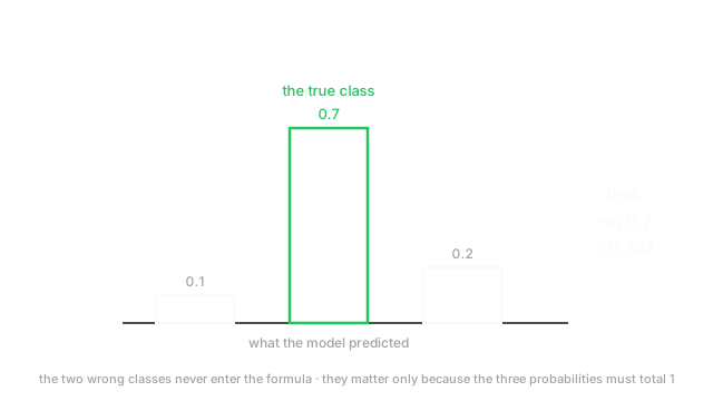
In plain words: the loss is the negative log of the probability assigned to the right answer, full stop. The predicted probabilities for wrong classes never appear in the formula — they matter only indirectly, because the softmax forces the total to 1, so raising the wrong ones lowers the right one.

That collapse is why the loss is often called negative log-likelihood, and why the implementation only needs to index one number per example.

Its relationship to entropy and KL divergence

Cross-entropy decomposes cleanly:

H(p, q) = H(p) + D_{\text{KL}}(p \parallel q)

In plain words: the cost of using $q$ splits into the uncertainty that was genuinely there plus the extra you pay for $q$ being wrong. Since $H(p)$ depends only on the data and not on your model, minimising cross-entropy and minimising KL divergence are the same optimisation.

This also explains why cross-entropy loss rarely reaches zero on real data. The floor is $H(p)$ , the irreducible uncertainty in the labels themselves. If two identical inputs carry different labels, no model can drive the loss below that, and chasing zero means memorising noise.

The gradient is the reason it is used

Pair a softmax output layer with cross-entropy loss and the gradient with respect to the pre-softmax logits is startlingly simple:

\frac{\partial \mathcal{L}}{\partial z} = \hat{y} - y

In plain words: predicted probabilities minus the one-hot target. That is the entire backward pass for the output layer.

Two things fall out of this. The gradient is proportional to the error, so a badly wrong prediction produces a large gradient and learning is fast where it needs to be — unlike mean squared error paired with a softmax, where the saturating exponential flattens the gradient exactly when the model is most wrong. And no derivative of the exponential survives in the final expression, which is why the two are always implemented as one fused operation.

Worked example

Three classes, the true class is the second one, so $y = [0, 1, 0]$ . The model predicts $\hat{y} = [0.1, 0.7, 0.2]$ .

Only the true class contributes:

\mathcal{L} = -\ln(0.7) \approx 0.357

Now the same true label with a worse prediction, $\hat{y} = [0.2, 0.2, 0.6]$ — the model is confident about the wrong class:

\mathcal{L} = -\ln(0.2) \approx 1.609

Four and a half times the loss, from the same label. And the gradient in the first case is $\hat{y} - y = [0.1, -0.3, 0.2]$ : push the true class up by 0.3, push the two wrong classes down. You can read the model's correction directly off the numbers.

A useful reference point: a uniform guess over 3 classes gives $-\ln(1/3) \approx 1.099$ . Any loss above that means the model is doing worse than knowing nothing, which is the first thing to check when a run looks broken.

Show Me the Code

1import numpy as np2
3
4def cross_entropy_from_logits(logits: np.ndarray, target: int) -> float:5    # log-sum-exp: subtract the max first so exp() can never overflow.6    shifted = logits - logits.max()                      # shape (n_classes,)7    log_probs = shifted - np.log(np.exp(shifted).sum())   # log softmax, stable8    return float(-log_probs[target])9
10
11probs = np.array([0.1, 0.7, 0.2])12print(-np.log(probs[1]))                          # -> 0.3566...  the true class13print(-np.log(np.array([0.2, 0.2, 0.6])[1]))      # -> 1.6094...  confidently wrong14
15logits = np.array([800.0, 802.0, 801.0])          # naive exp() would overflow here16print(cross_entropy_from_logits(logits, 1))       # -> 0.4076...17print(-np.log(np.exp(logits) / np.exp(logits).sum())[1])  # -> nan  (overflow)

The first two numbers match the hand calculation. The last pair is the point: identical mathematics, and only the stabilised version survives logits of realistic magnitude.

Watch Out For

Computing softmax and log separately

np.log(softmax(x)) and log_softmax(x) are the same function on paper and not in floating point.

Softmax exponentiates. A logit of 800 gives $e^{800}$ , which overflows float32 — whose ceiling is about $3.4 \times 10^{38}$ , reached at a logit of only 88. The result is inf, then inf/inf is nan, and the nan spreads through every gradient. In the other direction, a small probability underflows to exactly 0 and log(0) is -inf.

The fix is the log-sum-exp trick: subtract the maximum logit before exponentiating. Since softmax is unchanged by adding a constant to every logit, this is exact rather than an approximation — the largest exponent becomes $e^0 = 1$ , so nothing can overflow, and the logarithm is folded in algebraically instead of being applied to an already-lossy probability.

In practice this means always use the fused API: cross_entropy on raw logits, never nll_loss(log(softmax(x))) assembled by hand. If your model's final layer applies a softmax and your loss function expects logits, you have applied it twice — the symptom is a loss that starts near the uniform value and descends far too slowly.

Chasing a loss of zero

Cross-entropy's floor on real data is $H(p)$ , the entropy of the labels themselves, not zero. Any genuine label noise or inherent ambiguity puts a hard bound on how low the loss can go, and a training loss heading toward zero on a dataset with either means the model is memorising the noise.

The mechanism is worth understanding, because it is a stability problem as much as an accuracy one. Driving the predicted probability toward 1 requires the winning logit to run away toward infinity, since softmax only reaches 1 in the limit. So the weights grow without bound, the model becomes maximally overconfident, and calibration collapses: it reports 99.9% confidence on inputs it gets wrong.

Label smoothing is the standard answer — replace the one-hot target with something like 0.9 for the true class and the remaining 0.1 spread across the others. That gives the loss a finite minimum at finite logits, so there is nothing to run away toward. It costs a little raw accuracy and buys calibration and stability, which is usually the right trade when the probabilities themselves get used downstream.

The Quick Version

Cross-entropy is the average surprise of describing reality $p$ with your prediction $q$ : $-\sum p \log q$ .
With one-hot targets it collapses to $-\log q(\text{correct class})$ . Wrong-class probabilities never appear.
Confidently wrong is punished enormously; a probability of 0 on the true class costs infinity.
It decomposes as $H(p) + D_{\text{KL}}(p \parallel q)$ , so minimising it is minimising KL divergence.
The floor is $H(p)$ , not zero. Label noise sets a hard bound.
Paired with softmax, the gradient on the logits is just $\hat{y} - y$ — which is why they are fused.
Minimising cross-entropy is maximum likelihood under a categorical assumption.
Always compute from logits with log-sum-exp. Separate softmax and log overflow at a logit of 88 in float32.
Label smoothing gives the loss a finite minimum and stops logits running away.