Visual explainer

Feedback Control and PID

Trace error, proportional torque, retained integral effort and rate damping, then check saturation, conditional integration and derivative noise.

A feedback controller uses the measured gap from a target to adjust motor effort. PID combines present error, accumulated error and the rate of change of error. Those terms require suitable gains, a stable loop and explicit actuator limits.

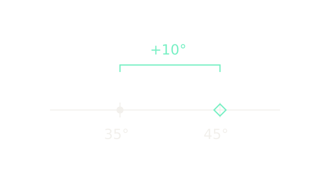
Error is the signed gap from measurement to setpoint.

The dot is a measured angle of 35 degrees; the diamond is the desired 45 degrees. On this cropped ruler, twenty pixels represent one degree. Their signed gap is $e=\theta_d-\theta=+10^\circ$ . Positive error asks this joint to increase its angle. A real loop repeatedly measures, computes effort, applies it and measures again.

Scale the current error

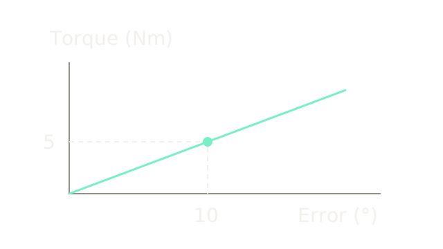
Proportional torque grows linearly with present error.

For a torque-controlled joint, $u_P=K_pe$ . Choose the illustrative gain $K_p=0.5$ Nm/degree. Ten degrees produces five newton metres; zero error produces zero P torque. The point and dashed projections locate this calculation on a graph with twenty pixels per degree horizontally and fifteen pixels per newton metre vertically. These gains are teaching values, not tuning advice.

Why does the joint droop?

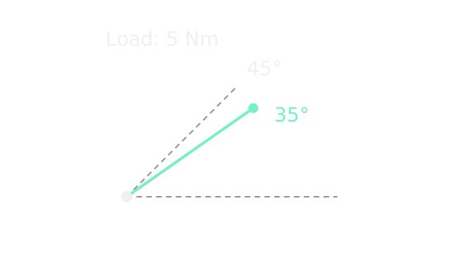
A constant load leaves a stable P-only joint below target.

The equal-length rays show an actual 35-degree arm and a dashed 45-degree target. Approximate the opposing load locally as a constant five newton metres. At a stable resting equilibrium without feedforward, motor effort must balance that load:

$K_pe_{ss}=\tau_{load},\qquad e_{ss}=5/0.5=10^\circ.$

This is a steady-state calculation, not a transient simulation. Gravity generally depends on configuration; the constant-load approximation applies around the operating posture. P-only effort needs a nonzero error to sustain a nonzero load.

Remember the past error

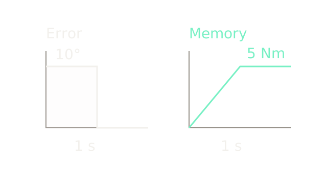
Stored integral torque remains after current error becomes zero.

The left trace is a deliberately simple input: ten degrees of error for one second, then zero. Its shaded area is ten degree-seconds. With $K_i=0.5$ Nm/(degree-second), the accumulated contribution $u_I=K_i\int e\,dt$ rises to five newton metres and stays there after the input becomes zero. Both horizontal axes use 100 pixels per second. The vertical scales differ: twelve pixels per degree on the left, twenty-four pixels per newton metre on the right.

This illustrates memory, not the arm's closed-loop response. In a stable, unsaturated PID loop, retained integral effort can balance a constant load at zero steady-state error. Excessive integral gain can instead destabilize the loop.

Oppose the measured rate

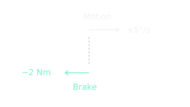
Derivative torque opposes measured motion at a fixed setpoint.

For a fixed target, $\dot e=-\dot\theta$ , so $u_D=K_d\dot e=-K_d\dot\theta$ . With $K_d=0.4$ Nm·s/degree and increasing angle at five degrees per second, D contributes minus two newton metres. The upper arrow represents rate; the lower represents torque. They use different units and separate scales, so compare their directions, not their lengths.

D reacts to a measured slope. It does not know the future or guarantee that overshoot disappears. Taking the derivative of measurement instead of error also avoids the derivative kick caused by a setpoint step; practical implementations usually filter the rate estimate.

Add signed contributions

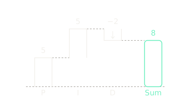
Signed PID contributions sum to the requested torque.

The waterfall adds P = 5 and I = 5, then subtracts two from D, yielding a requested eight newton metres. All vertical lengths use twenty pixels per newton metre. Floating bars show increments; the final bar starts at zero. This is an illustrative snapshot with integral memory already present.

$u=K_pe+K_i\int e\,dt+K_d\dot e.$

A discrete implementation updates the integral with $e_k\Delta t$ and estimates rate using $(e_k-e_{k-1})/\Delta t$ . Sampling, gain units, filtering and initialization must agree with that implementation.

Specify the response model

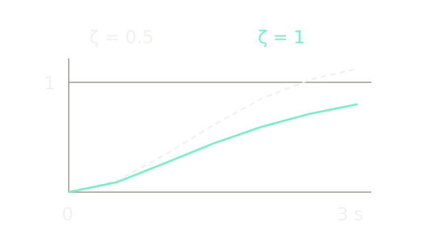
Two specified damping ratios give different normalized step responses.

This frame deliberately introduces a separate ideal second-order model, $G(s)=1/(s^2+2\zeta s+1)$ , with unit natural frequency and a unit step. It does not simulate the loaded joint above. Dashed uses damping ratio $\zeta=0.5$ ; solid uses $\zeta=1$ . Both curves are analytic samples at half-second intervals, connected by straight segments. Horizontal scale is 140 pixels per second; output one lies 160 pixels above zero.

The critical response is $y(t)=1-(1+t)e^{-t}$ . The underdamped response is $y(t)=1-e^{-t/2}[\cos(bt)+(0.5/b)\sin(bt)]$ , with $b=\sqrt{0.75}$ . At three seconds the outputs are approximately 0.80085 and 1.12435. The dashed trace has crossed the target; the solid trace has not. These results depend on the specified model. They do not establish a universally fastest or optimal PID tuning.

Respect motor effort limits

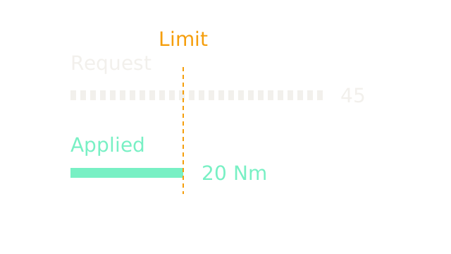
A torque limit clips requests beyond twenty newton metres.

With a hypothetical limit of $\pm20$ Nm, $u_{applied}=\operatorname{clip}(u_{requested},-20,20)$ . A 45 Nm request becomes 20 Nm. The two bars share eight pixels per newton metre, making the clipping visible. The controller still receives feedback; saturation makes its input-output behavior nonlinear, rather than opening the feedback connection.

Let the integral unwind

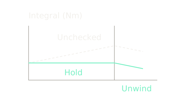
Conditional integration blocks growth but still permits unwinding.

This accumulator fixture starts with I = 20 Nm. Three one-second intervals of positive error would add five newton metres each, taking an unchecked I to 25, 30 and 35. Conditional integration holds it at 20 while those updates would drive an upper-saturated request farther out. In the last interval error becomes negative, reducing the unchecked value to 30 and the conditional value to 15. Each second occupies 100 pixels; each newton metre occupies four pixels vertically.

A simple rule blocks an integral increment when the request is at or beyond a bound and the increment pushes farther beyond that bound. It permits increments that unwind saturation. Freezing every saturated update can prevent recovery. Back-calculation is another option, using the difference between requested and applied effort. These example traces show integral state under prescribed conditions, not a complete plant response or a guarantee against all overshoot.

Where it breaks

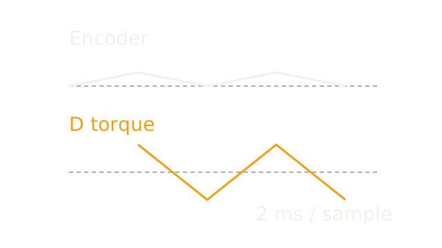
Differentiating encoder jitter creates large alternating torque requests.

The top trace is an error signal alternating between zero and 0.1 degrees every two milliseconds. Backward differences alternate between plus and minus $0.1/0.002=50$ degrees per second. Multiplying by $K_d=0.4$ produces alternating D requests of plus and minus 20 Nm, shown from the second sample onward. The top uses 200 pixels per degree; the bottom uses two pixels per newton metre. Dotted lines mark zero in each trace; the vertical units differ.

A small position fluctuation can thus demand substantial effort. A filtered derivative reduces high-frequency sensitivity at the cost of lag; sensor quality and sampling also matter. This calculation predicts a controller request, not gearbox damage or the motor's realized high-frequency torque.

The Quick Version

Error subtracts the measured state from the target.
Proportional effort scales the current error.
A constant load can leave P-only control with offset.
Integral memory can supply holding torque at zero error.
Derivative action opposes motion for a fixed target.
PID adds signed contributions before actuator limiting.
Response claims require a specified plant and gains.
Saturation clips effort while feedback remains connected.
Anti-windup should permit integration that reduces saturation.
Differentiation amplifies sample-to-sample noise; filtering adds lag.

Sources

Modern Robotics, torque-input control supports the load-offset and integral-stability discussion. MathWorks anti-windup documents saturation and recovery methods. Control Station on derivative measurement explains the rate sign and setpoint kick. Numerical fixtures here are synthetic.