State Estimation and the Kalman Filter

A state estimator combines a motion model with observations to infer a robot's state. Here a scalar Kalman filter estimates position on a line, keeping both a mean and a variance. Its uncertainty is meaningful only insofar as the model and noise assumptions fit the situation.

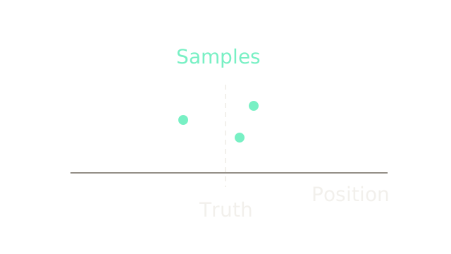
The synthetic true position is 2.2 metres, shown as a dashed reference unavailable to the estimator. Observations at 1.6, 2.4 and 2.6 metres disagree. Horizontal location encodes position at 100 pixels per metre; vertical offsets only separate the samples. This opening illustration motivates uncertainty; the worked filter below starts with its own specified prior.

Start with a belief

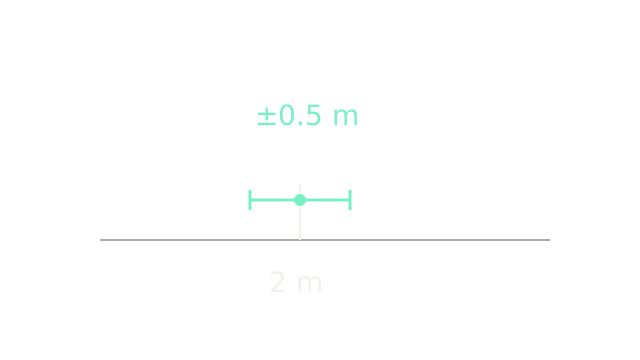
Set initial mean $m_0=2.00$ m and variance $P_0=0.25$ m². The corresponding standard deviation is $\sqrt{P_0}=0.50$ m. The dot marks the mean; the interval spans mean plus or minus one standard deviation, from 1.50 to 2.50 metres. It is not a bound containing every possible position. Throughout these interval drawings, endcaps identify spread, not walls.

Predict the next position

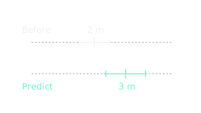
Use $x_1=x_0+u_1+w_1$, with known displacement input $u_1=1$ m and independent zero-mean process noise of variance $Q=0.15$ m². Then

$m_1^-=2+1=3.00\text{ m},\qquad P_1^-=0.25+0.15=0.40\text{ m}^2.$

The two rows share 100 pixels per metre. The predicted mean shifts right by 100 pixels and its interval halfwidth grows from 50 to $100\sqrt{0.40}=63.246$ pixels. This growth follows from the additive model with positive Q; covariance need not increase under every state-transition model.

Receive an observation

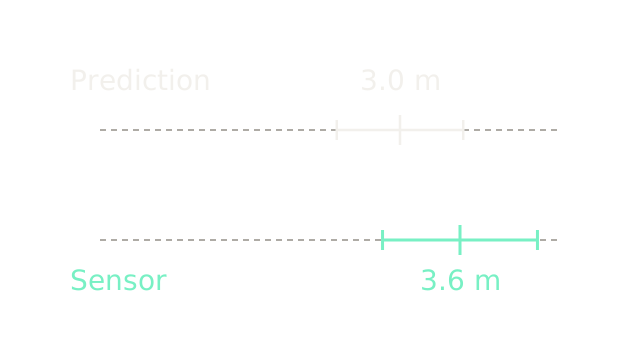
Assume a calibrated position observation $z_1=x_1+v_1$, with independent zero-mean noise variance $R=0.60$ m². Let the received value be 3.60 metres. Its noise standard deviation is $\sqrt{0.60}=0.774597$ m, larger than the prediction's 0.632456 m. The lower interval is centered on the observed value to visualize this noise scale; it is not a second posterior distribution.

A raw distance to a wall must first be mapped into the chosen position coordinate with the correct origin and sign. Here that conversion is already included in z; no velocity or orientation state is being estimated.

Measure the disagreement

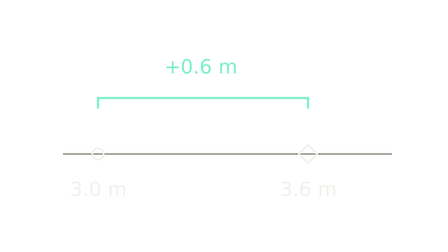
This detail view zooms to 500 pixels per metre. The ring is prediction, the diamond observation. Their separation is $\nu_1=z_1-m_1^-=3.60-3.00=+0.60$ m, shown by a 300-pixel bracket. Innovation variance is $S_1=P_1^-+R=1.00$ m². A positive residual means the observation is ahead of the prediction; it does not prove the robot really moved that extra distance.

Compute the correction weight

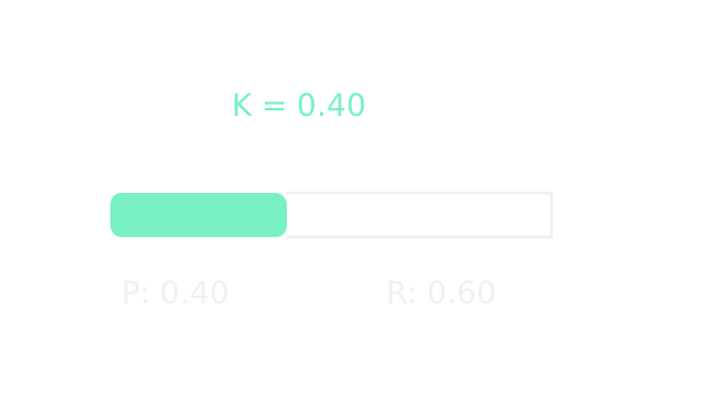
The variance bar divides $P_1^-=0.40$ and $R=0.60$ at 400 pixels per square metre. The first segment occupies forty percent of the total. For this scalar direct-observation model,

$K_1=\frac{P_1^-}{P_1^-+R}=0.40.$

This is a correction weight derived from specified uncertainties, not a claim that forty percent of the residual is true motion. The scalar weight lies between zero and one for positive finite variances; general matrix gains are not restricted elementwise to that interval.

Move partway toward the observation

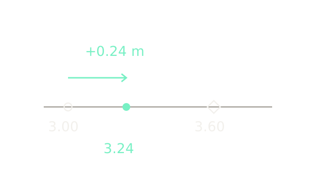
The 500-pixels-per-metre zoom matches frame five. The filled posterior dot lies 120 pixels beyond the prediction, forty percent of the 300-pixel gap:

$m_1=m_1^-+K_1\nu_1=3.00+0.40(0.60)=3.24\text{ m}.$

The remaining 0.36 metres to the observation is deliberately not applied. An arithmetic average would give 3.30 metres; these unequal variances produce a different weight.

Compare uncertainty widths

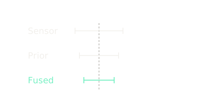
The intervals are deliberately recentered to compare width at 100 pixels per metre, so their centers no longer show different position means. Sensor, prediction and posterior halfwidths are 77.460, 63.246 and 48.990 pixels.

$P_1=(1-K_1)P_1^-=0.60(0.40)=0.24\text{ m}^2.$

For this scalar independent-noise model with positive finite variances, $P_1=P_1^-R/(P_1^-+R)$ is smaller than either input variance. That does not mean each realized estimate is closer to truth. Correlated errors or a misspecified noise model invalidate this calculation's interpretation.

Reuse the posterior

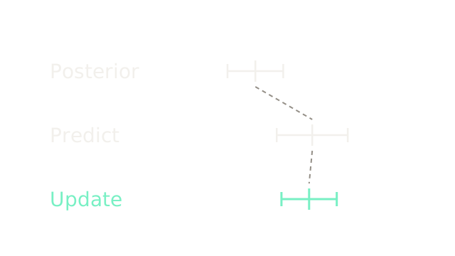
Now zoom out to 80 pixels per metre. Begin with mean 3.24 and variance 0.24. Another one-metre input gives predicted mean 4.24 and variance $0.24+0.15=0.39$. Receive $z_2=4.10$ m. The gain is $0.39/(0.39+0.60)=13/33$, giving

$m_2=4.24+\frac{13}{33}(4.10-4.24)\approx4.184848\text{ m},\qquad P_2\approx0.236364\text{ m}^2.$

The final interval contracts and its center shifts slightly left. Dashed connections trace the carried mean. Fixed-dimensional mean and covariance summarize the prior observations; the recursion does not require storing the entire history. It does not guarantee rejection of spikes or bounded actual error under arbitrary operating conditions.

Where it breaks

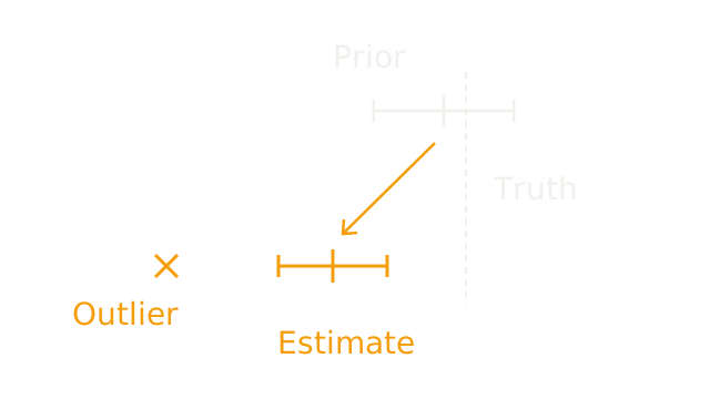
Return to the first prediction, mean 3.00, variance 0.40, and the 100-pixels-per-metre scale. Replace the observation by a glitch at 0.50 metres. The same gain yields $3+0.4(0.5-3)=2.00$ metres. Assume synthetic ground truth 3.20 metres: the update moves away from it. Yet the reported variance remains 0.24, because this covariance update does not depend on the observed value. The narrower amber interval excludes the displayed truth without detecting the glitch.

The exact Gaussian posterior interpretation requires a linear model, Gaussian prior and correctly specified independent Gaussian noises. Innovation checks, sensor diagnostics or robust observation models can help with outliers; a particle filter alone does not automatically reject them. Underestimated process noise can also make confidence misleading. Nonlinear models need an appropriate estimator, such as an EKF or UKF approximation, with their own limits.

The Quick Version

• Observations can disagree with the same underlying physical state.
• A scalar belief stores mean position and position variance.
• This additive prediction shifts the mean and adds process variance.
• Measurement noise has its own variance in observation coordinates.
• Innovation measures disagreement, not verified extra motion.
• Kalman gain weights the correction using specified uncertainties.
• The worked update moves 3.00 metres to 3.24 metres.
• Posterior covariance describes model uncertainty, not guaranteed actual accuracy.
• Each posterior seeds the next prediction and update.
• Outliers can mislead an estimate while reported covariance contracts.

Sources

Särkkä, Bayesian Filtering and Smoothing, chapter 4.3 gives the linear-Gaussian model, recursion and random-walk example. The scalar Kalman gain derivation details the variance weighting. All numerical inputs and illustrations here are synthetic.