Motion Planning

Motion planning finds a route that respects the robot's geometry and obstacles. Executing that route also requires timing, motion constraints and feedback. A path found on a static map remains a proposal until those conditions are checked.

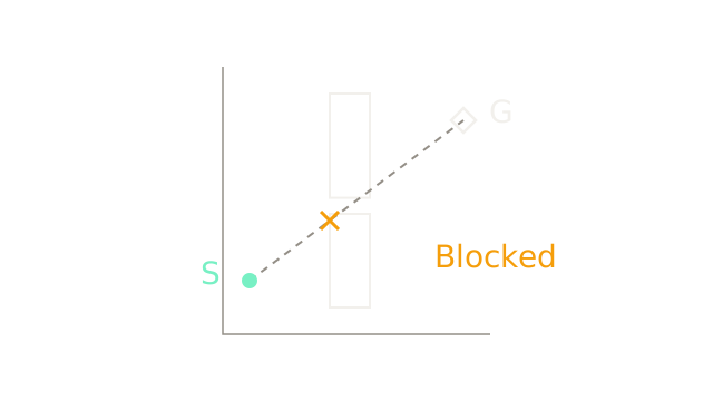
The synthetic ten-by-ten-metre workspace starts at $S=(1,2)$ and ends at $G=(9,8)$. Two rectangular barriers share x bounds $[4,5.5]$ m; their y bounds are $[1,4.5]$ and $[5.1,9]$ m. The drawing uses the same 24 pixels per metre in both directions, with world y pointing up.

The direct segment follows $y=0.75x+1.25$. At the first barrier's left face, $x=4$, it reaches $y=4.25$, inside that barrier. The cross marks this intersection. Pointing toward the goal does not establish a clear route.

Account for the whole body

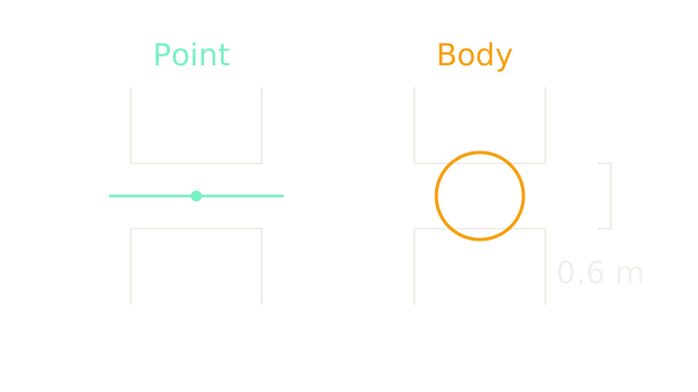
Zoom into the facing surfaces at 100 pixels per metre. Their separation is $5.1-4.5=0.60$ m. A circular body of radius 0.40 m has diameter 0.80 m. A point passes through the opening; the circle overlaps each surface by 0.10 m when centered in it. These paired cutaways show the passage interior, not the full barriers.

The robot's center can be in empty workspace while its body collides. Body geometry must participate in the collision test.

Inflate the forbidden region

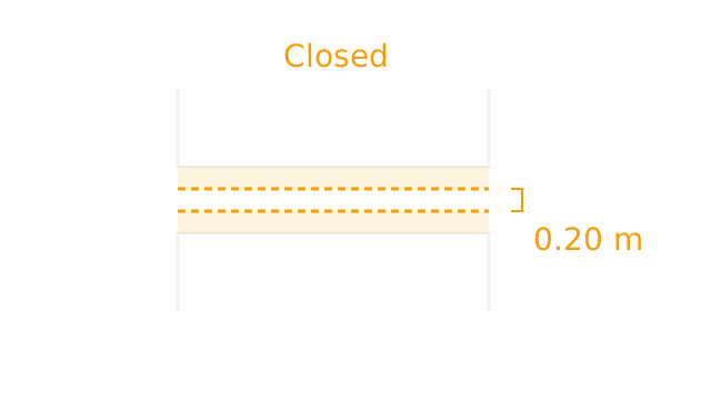
For this translating circular robot, grow obstacles by its radius and plan for its center as a point. The forbidden center positions form the Minkowski sum $\mathcal C_{obs}=\mathcal W_{obs}\oplus\mathcal B_{0.4}$. Actual rectangle corners become rounded; the diagram isolates the flat interior faces, so its vertical cuts are not outer obstacle edges.

The lower barrier's upper forbidden boundary reaches $4.5+0.4=4.9$ m. The upper barrier's lower forbidden boundary reaches $5.1-0.4=4.7$ m. Their overlap is 0.20 m, drawn as twenty pixels. The passage is closed. For a rotating noncircular body or an arm, configuration space also includes orientation or joint coordinates; uniform planar inflation alone is insufficient.

Define a finite grid

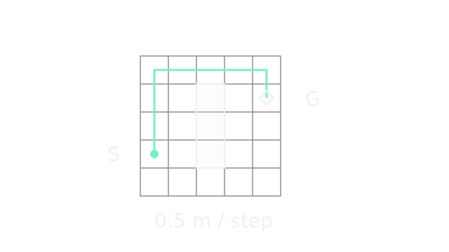
For a checkable search example, switch to a separate five-by-five configuration-space grid, with half-metre cells and four-neighbor moves. Label cell centers by integer indices $(i,j)$, starting at the bottom left. Start is $(0,1)$, goal $(4,3)$, and cells $(2,1)$, $(2,2)$ and $(2,3)$ are blocked. This is a discrete example, not a rasterization of the previous map.

The illustrated upper route takes three steps up, four right and one down: eight steps, four metres. A valid edge must also be collision-free between its endpoint configurations. Conservative occupancy can mark every cell intersecting an inflated obstacle as blocked, at the cost of excluding some narrow valid passages. Grid resolution and allowed moves define which paths can be found.

Add traveled and remaining costs

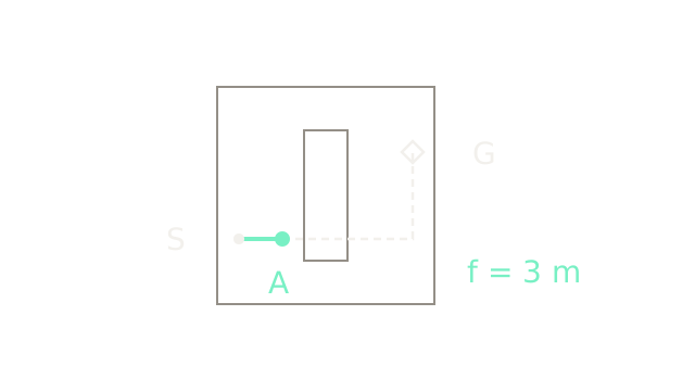
At candidate A = $(1,1)$, the solid prefix is one half-metre step from S, so $g(A)=0.5$ m. Use Manhattan distance as an optimistic remaining cost on this four-neighbor grid:

$h(A)=0.5(|4-1|+|3-1|)=2.5\text{ m},\qquad f(A)=g(A)+h(A)=3.0\text{ m}.$

The dashed five-step lower-bound route crosses a blocked cell. It illustrates the heuristic's deliberate omission of obstacles; it is not an accepted motion. The actual remaining path must detour.

With nonnegative edge costs, a consistent heuristic and correct search bookkeeping, A* returns a shortest path on this graph. An admissible but inconsistent heuristic generally requires reopening improved nodes. Neither condition establishes a shortest path in the underlying continuous world. A weak heuristic can still leave substantial exploration.

Expand a cheapest frontier candidate

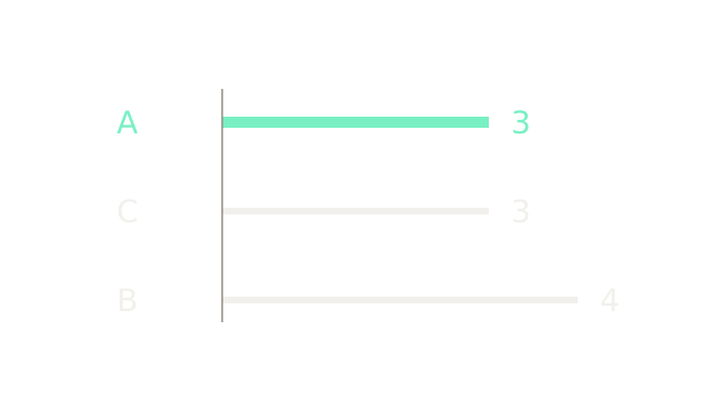
Immediately after expanding S, A = $(1,1)$ and C = $(0,2)$ each have $g=0.5$, $h=2.5$ and $f=3$ m. B = $(0,0)$ has $g=0.5$, $h=3.5$ and $f=4$ m. Shared-scale bars show these priorities at eighty pixels per metre. A stable tie rule may choose A or C first; the mint bar illustrates choosing A.

For each valid neighbor, compute a tentative traveled cost. If it improves that node's best known g, update the cost and parent and refresh its queue priority. Previously discovered nodes may need improvements; merely inserting unseen neighbors is insufficient. Terminate according to the algorithm's goal-removal condition, then reconstruct through parent links.

Extend a sampled tree

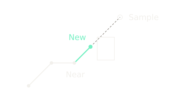
This separate two-dimensional configuration example illustrates a geometric RRT step. Existing vertices are $(0,0)$, $(1,1)$ and $(2,1)$; the sample is $(4,3)$. Under Euclidean distance, the nearest vertex is $(2,1)$, at distance $\sqrt8$. A unit-length extension gives

$q_{new}=(2,1)+\frac{(2,2)}{\sqrt8}\approx(2.707107,1.707107).$

At eighty pixels per coordinate unit, the new solid edge is exactly eighty pixels long. The dashed remaining ray toward the sample crosses an obstacle, but that portion is not added. Check the full proposed edge before adding it, not just the new endpoint.

Sampling avoids explicitly filling a high-dimensional grid: fifty bins across seven joints would require $50^7=781{,}250{,}000{,}000$ cells. It still depends on collision checks, an appropriate distance metric and a local planner. Completeness statements are asymptotic and conditional on sampling, clearance and steering assumptions; finite samples do not guarantee success or an optimal path.

Give the path a clock

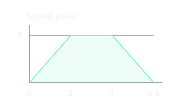
Now consider a separate straight four-metre translation, starting and ending at rest. With speed at most 1 m/s and acceleration magnitude at most 0.5 m/s², accelerate for two seconds, cruise for two, then brake for two. The area under the speed trace is $1+2+1=4$ metres. The plot uses seventy pixels per second and 160 pixels per m/s.

A geometric path $q(s)$ becomes a trajectory through a time law $s(t)$. This trapezoid gives continuous velocity but discontinuous acceleration at phase boundaries, so jerk is not bounded there. It satisfies the stated one-dimensional limits; it does not prove motor-torque, steering, curvature or obstacle feasibility for an arbitrary robot. Following a sharp corner at nonzero speed would require an instantaneous direction change. Stopping at the corner is another option; rounding it changes the path and requires new checks.

Recheck every smoothed segment

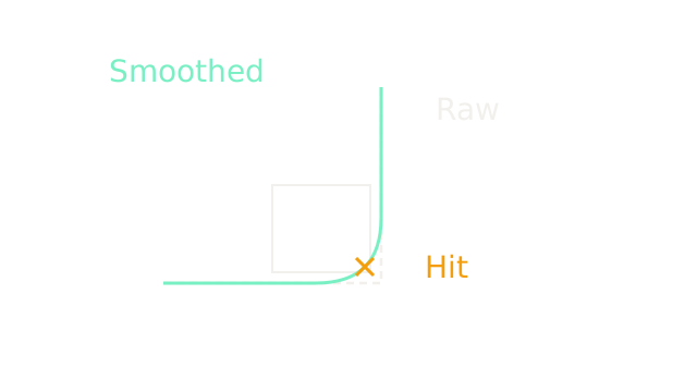
This new configuration-space patch makes the risk explicit. The dashed L path runs from pixel $(150,260)$ through $(350,260)$ to $(350,80)$. It clears the already inflated rectangle $[250,340]\times[170,250]$. Replace its corner with a quadratic Bézier from $(290,260)$ through control point $(350,260)$ to $(350,200)$. At parameter one half, the curve is $(335,245)$, inside the rectangle; the cross marks that collision.

Smooth-looking geometry does not establish collision freedom or bounded steering. Revalidate the entire curve, its timing and relevant dynamics. Position differentiability is also not the same as curvature continuity. Feedback tracking then follows a feasible reference and compensates for disturbances; it cannot make an unsafe reference safe by definition.

Where it breaks

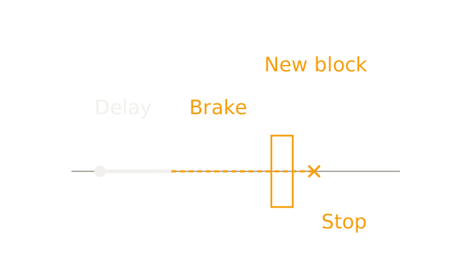
A previously clear route can become blocked. In this synthetic one-dimensional stopping example, the robot travels at 1 m/s, takes 0.5 seconds to react and can brake at 0.5 m/s². Distance to stop is

$d=v\Delta t+\frac{v^2}{2a}=1(0.5)+\frac{1}{2(0.5)}=1.5\text{ m}.$

The new inflated obstacle begins only 1.2 metres ahead of the current center. At 200 pixels per metre, reaction travel is 100 pixels and braking travel 200; the hypothetical unobstructed stopping point lies past the boundary. This is an unsafe stopping scenario, not an executed path through an obstacle or a measured planner benchmark.

A static route alone cannot manage this change. Execution needs updated sensing and collision checks, sufficient clearance, and a response policy consistent with available braking and motion constraints. A replanner returning later cannot recover already consumed stopping distance.

The Quick Version

• A direct start-to-goal line can intersect obstacles.
• Collision checks must include the robot's body.
• Configuration-space obstacles represent forbidden robot configurations.
• Grid resolution and allowed moves define the search graph.
• A* combines traveled cost with an optimistic remaining cost.
• Frontier ties and improved paths require explicit bookkeeping.
• RRT adds checked local extensions, not unchecked sample connections.
• Time scaling must satisfy the relevant motion constraints.
• Smoothing can introduce collisions between safe waypoints.
• Delay consumes clearance before braking even begins.

Sources

Modern Robotics explains C-space obstacles, A* graph search, RRT extension and path time scaling. The numerical maps, curves and stopping example here are synthetic.