Robot Learning: Imitation to RL

Robot learning fits a policy that maps observations to actions. Imitation learning uses expert examples; reinforcement learning uses rewards from interaction. Both still need feedback, suitable training data, and a task specification that matches the intended outcome.

1. Contact Changes Motion

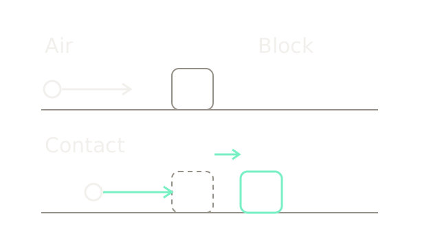
The upper pusher moves through air; the block stays put. In the lower view, contact transmits motion. The dashed square marks the old block position and the solid square its new position. Both views use the same scale: a long arrow represents a 2 cm command. The short arrow identifies the block's change of position, rather than another measured command.

Our synthetic task is to push a block from x = 0 to x = 10 cm. Assume ideal tracking for the worked arithmetic. Real displacement depends on friction, contact geometry and compliance. Analytical contact models exist; learning is useful when fitting behavior from interaction is easier than identifying every model parameter. It does not remove the physics.

2. Pair Observations With Actions

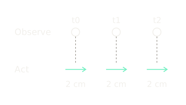
Each dashed column pairs an observation with the expert command at that timestamp. Here three observations have the same 2 cm forward command. Observations might contain an image, joint positions and the previous action; actions must have a defined frame, unit and timing convention.

Record aligned pairs rather than only the final successful trajectory. Teleoperation is one collection method, as in ACT's demonstration setup. Logging rates and trial lengths determine dataset size: fifty trials alone say nothing about the number of recorded pairs.

3. Fit The Demonstrated Actions

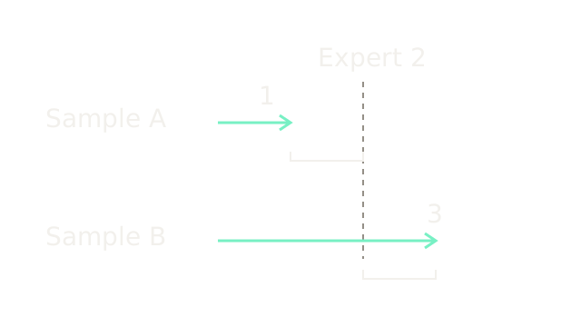
The dashed reference is the expert's 2 cm command. Predicted arrows have lengths 1 and 3 cm. Equal brackets mark their equal absolute errors. Behavior cloning adjusts the policy to reduce a supervised loss on such pairs; the drawing shows the residuals it trains against, not an already completed update.

For this scalar example, mean squared error is:

$$L = \frac{(1-2)^2 + (3-2)^2}{2} = 1\;\mathrm{cm}^2.$$

Mixed action dimensions need explicit normalization or weighting. A small held-out imitation loss tests predictions on that dataset; it does not establish that the robot will recover from mistakes during execution.

4. Actions Change Future Inputs

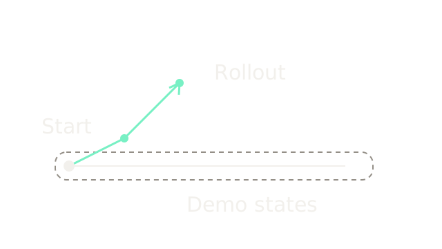
This plan view changes the scale to 40 drawing units per centimetre on both axes. The dashed band represents demonstration pusher positions within 0.5 cm of the centerline. The learner visits (0, 0), (2, 1), then (4, 3) cm and leaves that coverage. These are deliberately chosen illustrative positions, not predictions of a physical error-growth law.

An action affects the next observation, so a small mistake can create an input absent from training. The DAgger paper analyzes this sequential dependence. Its quadratic worst-case cost dependence under behavior-cloning assumptions does not mean lateral distance must grow quadratically in every robot rollout.

5. Label The Visited State

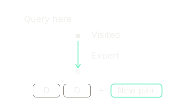
Keep the preceding plan-view scale. At the visited position (4, 3) cm, the expert labels a recovery command of (0, −3) cm. Under the ideal displacement assumption, that command returns the pusher to (4, 0). The open circle is the recovery endpoint. The lower row represents old dataset samples plus this new observation–expert-action pair; its spacing has no physical scale.

DAgger repeatedly collects states encountered by the learner, queries expert actions there, adds those pairs to the dataset and retrains. Expert mixing may help collect rollouts; a knowledgeable expert and feasible recovery states remain assumptions. The label is the expert's action at the visited state, not the learner's mistaken action. Coverage can improve without guaranteeing recovery everywhere.

6. Score Transitions With Reward

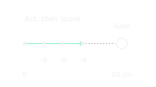
Return to the block's forward coordinate. Points at x = 0, 2, 4 and 6 cm show three executed transitions, with a goal ring at 10 cm. Let reward be negative remaining distance in centimetres after each action. The three rewards are −8, −6 and −4, giving an undiscounted three-step return of −18. A fourth action to x = 8 would receive −2, bringing that four-step sum to −20; longer negative-return sums require consistent horizons when comparing policies.

Reinforcement learning searches for policies with higher expected return. More generally the objective is the expected sum of discounted rewards, with discount factor γ. Rewards evaluate outcomes; they do not supply an expert command at every state. RL may start from demonstrations or an imitation-trained policy, so imitation and RL can be combined.

7. Exploration Has Physical Consequences

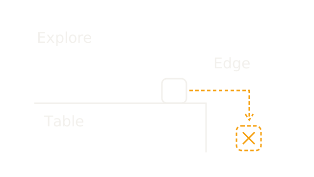
The dashed proposed path carries the block beyond its support. The cross marks an invalid physical outcome. This side-view schematic illustrates a failure condition; it does not simulate the block's falling trajectory.

Collecting interactions on hardware costs elapsed time, resets and wear, and unconstrained exploration can cause damage. Those costs vary with the task and training method. Neither a universal interaction budget nor inevitable motor destruction follows from using RL. Exploration limits, supervision and reset design belong to the learning setup.

8. Collect Parallel Simulated Rollouts

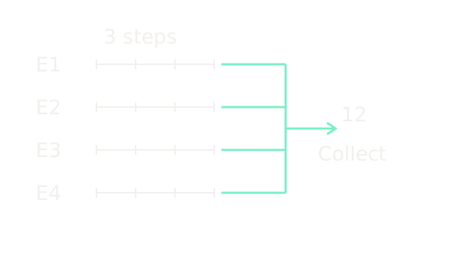
E1 through E4 are separate simulated environments. Four state marks delimit three transitions on each trace. The collection bus gathers 4 × 3 = 12 transitions for learning. Horizontal spacing is categorical timestep order, not centimetres or wall-clock time.

Simulation permits resets and parallel collection without exercising the real mechanism for each trial. It also has simulation, inference and update costs. Twelve transitions here establish a count, not a speedup or a training-time guarantee. Learned behavior may exploit errors in the simulated dynamics.

9. Vary The Simulated Dynamics

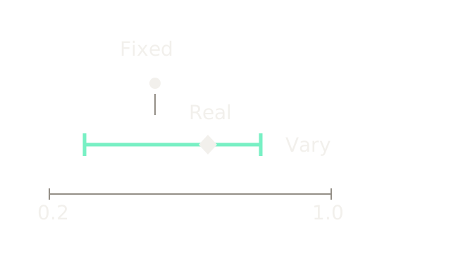
The horizontal axis is a dimensionless friction coefficient. Fixed training uses 0.5; randomized training samples the interval [0.3, 0.8]. The diamond at 0.65 lies inside that interval. Vertical separation distinguishes the two training setups and does not encode another physical variable.

Dynamics randomization trains across varied simulator parameters to improve transfer. These numbers are illustrative choices, not a prescription. A real coefficient of 0.9 falls outside our range. Even 0.65 being inside does not prove success: unmodelled contact, delay, perception error or interactions between parameters may still break the policy.

10. Where It Breaks

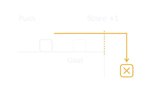
Now deliberately replace the distance reward with a flawed one: award +1 once the block touches the table boundary. The intended task is still placement at the dashed goal on the surface. The amber path crosses the scored boundary and loses the block, so it satisfies the proxy without completing the intended task. This is a constructed counterexample, not a reported robot experiment.

Changing observations can also invalidate an imitation policy's training coverage. The outcome depends on the policy and disturbance; a shadow does not imply that all neural activations become zero. Check the actual task outcome, test recovery under relevant shifts and constrain physical execution. More training on an incomplete reward or an unrepresentative simulator need not repair either failure.

The Quick Version

• Contact determines how commands move objects.
• Demonstrations pair observations with expert actions.
• Behavior cloning fits actions on those observations.
• Rollouts can leave demonstration coverage.
• DAgger collects expert labels at visited states.
• Reinforcement learning optimizes expected reward.
• Physical exploration needs constraints and reset design.
• Parallel simulations collect separate transitions.
• Randomized dynamics broaden training coverage without guaranteeing transfer.
• A high proxy reward can hide task failure.