Visual explainer
Vision-Language-Action Models
Follow an instruction and camera observation into robot actions, then compare action bins, continuous generation, chunk execution, and feedback limits.
A vision-language-action model predicts robot actions conditioned on images and a language instruction. Its learned policy connects task meaning with behavior. The action representation, training distribution and execution system determine what those predictions can accomplish.
1. Ground The Requested Motion
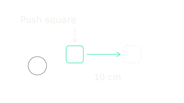
“Push square” selects the solid square rather than the circular distractor. The dashed square marks a desired location 10 cm to the right, not a second object. This is a schematic of the task relation; an image alone does not supply calibrated centimetres.
A VLA uses both the instruction and observation to predict an action. The picture does not imply that every VLA explicitly outputs a bounding box or reconstructs coordinates before acting. The command frame, calibration and robot interface still need a defined meaning. Our worked task keeps this square-pushing objective throughout, while later panels zoom into representations and timing.
2. Condition On Images And Words
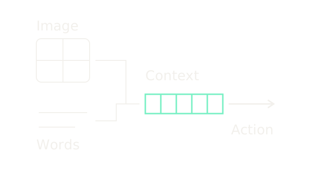
The patch grid and word strips enter a shared context ribbon. Cells stand for learned representations, not physical objects or attention weights. The arrow leaving the ribbon is an action prediction.
OpenVLA adapts a pretrained vision-language backbone using robot action data. Its model predicts discrete actions. Other VLAs add continuous action heads and may also condition on robot state or observation history. Pretraining provides representations; robot data establishes how outputs correspond to commands. A common diagram does not make these architectures identical.
3. Quantize An Action Coordinate
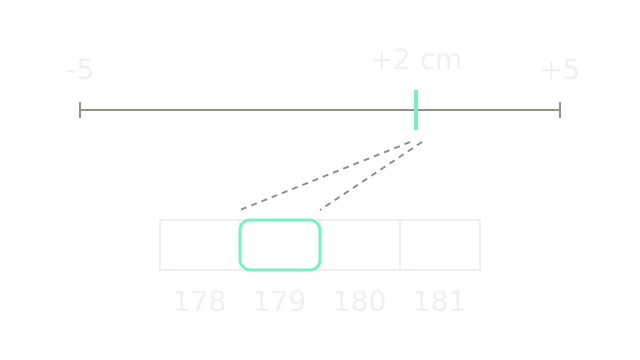
The top bar spans −5 to +5 cm for a single forward action coordinate. Its mint mark is +2 cm, 70% along the interval. Dashed leaders open a local zoom of four neighboring cells; the enlarged cell widths no longer share the top bar's physical scale.
For an ideal teaching quantizer with 256 equal cells, normalize and select a zero-based cell:
Clamp b to 0–255 at the endpoints. The cell width is 10/256 = 0.0390625 cm, or 0.390625 mm. Decoding to its center gives:
The representation error is 0.1171875 mm here. This says nothing about physical tracking accuracy. A +1 cm input maps to cell 153 and center 0.99609375 cm under the same convention.
OpenVLA discretizes normalized action dimensions, but this ideal equal-cell example is not a transcription of its implementation. Its tokenizer source uses digitization edges, clipping, bin-center decoding and a reverse mapping into vocabulary entries. Dataset statistics set action normalization. A cell index is not the resulting vocabulary token ID; inspect the exact implementation when reproducing its outputs.
4. Generate Continuous Actions
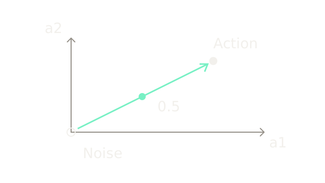
These axes are two action coordinates, not the tabletop. The open circle is an illustrative noise sample (0, 0); the target action is (2, 1). At interpolation time τ = 0.5, their straight training interpolation is (1, 0.5), the middle dot. For this pair, the target velocity is (2, 1). Flow time describes generation, not elapsed robot motion.
π0's method trains an action expert to predict a conditional velocity field. At inference it integrates that field from sampled noise to an action chunk. One training pair's straight interpolation illustrates the objective; it is not the complete learned field. Continuous generation avoids this scalar binning scheme, but does not guarantee submillimetre tracking, collision avoidance or correct behavior.
Diffusion Policy instead learns conditional denoising diffusion for action generation. Both can represent multiple plausible behaviors. Autoregressive discrete policies can also model multimodal distributions; multimodality is not exclusive to continuous heads.
5. Predict A Chunk
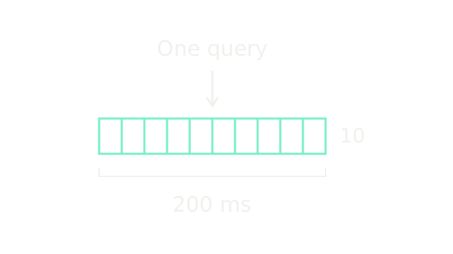
Each cell is one future command. In our synthetic schedule, ten commands consumed at 50 Hz cover 10/50 = 0.2 seconds, or 200 ms. Cell position encodes execution order, not displacement. ACT is a primary example of learning action chunks from demonstrations.
The policy must finish a usable prediction before the buffer needs it. Chunking can amortize computation, but the first chunk still takes time to compute, and a longer open-loop prefix delays reaction to new observations. Smooth motion also depends on the action representation and controller; predicting ten cells alone does not guarantee it.
6. Track At Another Rate
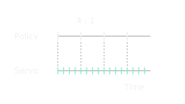
The aligned rows share a time axis. Four policy periods contain sixteen servo periods: an illustrative 4:1 rate ratio. Tick marks are update events. This simplified ratio replaces the preceding numeric schedule for clarity; it is not a reported VLA controller frequency.
A low-level controller uses current robot measurements to track commands between policy updates. It may interpolate setpoints and solve kinematic mappings, depending on the interface. Faster tracking feedback does not give the slow policy a new camera observation or repair a wrongly grounded instruction. Policy inference, command consumption and servo feedback are distinct clocks.
7. Interpret The Action Frame
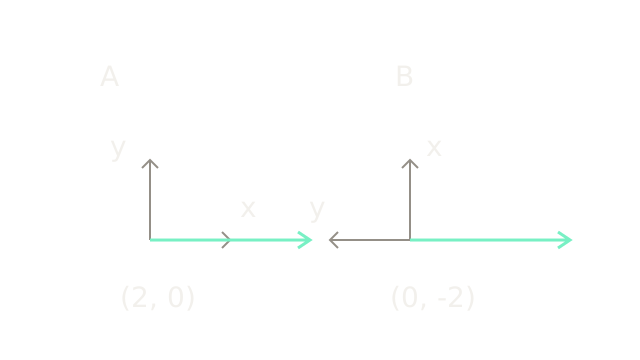
The mint vectors describe the same world-right displacement of 2 cm. A's local axes align with the world, so its action is (2, 0). B's axes are rotated 90 degrees counterclockwise: local x points up, local y points left. The same displacement is therefore (0, −2) in B. Arrow lengths share an 80 drawing-unit-per-centimetre scale.
This frame conversion is a small necessary example of making heterogeneous data interpretable. Shared training also needs consistent units, action semantics, sensor conventions and robot-specific interfaces. Joint limits, morphology and reachable workspaces still differ. Normalization alone does not make a learned policy transfer between embodiments; evaluate or adapt it on the intended robot.
8. Replan From Fresh Observations
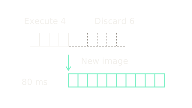
Return to the ten-action, 50 Hz schedule. Execute the first four commands, covering 4/50 = 80 ms; discard the remaining six when a fresh prediction replaces them. The lower chunk begins at that fourth-step boundary and predicts another 200 ms. Both rows share a time scale; the connecting arrow denotes a new observation and policy query, not instantaneous computation.
This is receding-horizon execution, conditional on the fresh chunk being ready. If inference takes longer than the chosen execution prefix, the system needs another scheduling strategy. The diagram does not claim an 80 ms replanning interval on arbitrary hardware.
Temporal ensembling, used in ACT, instead combines overlapping predictions for a given execution time. It may coexist with chunked execution, but averaging predictions and replacing an unexecuted suffix are different operations. Neither guarantees timely obstacle response.
9. Test A Changed Scene
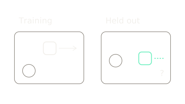
The held-out window moves the square and distractor while retaining object shapes and drawing scale. Its dashed proposed action ends in a question, because this is an evaluation design, not an observed success. The requested operation remains a rightward push of the square.
Test target selection, actual displacement and task completion under defined changes to layout, appearance and instruction wording. Record failures as well as successes. Useful pretrained representations may support transfer, but neither this sketch nor a model's language fluency establishes success in an unseen kitchen. Frame 1's metric task still requires appropriate calibration and execution.
10. Where It Breaks
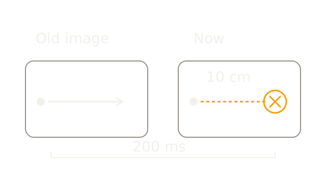
The old image shows a clear command corridor. In the current scene, a new obstruction occupies its endpoint. The dashed command continues from stale information and reaches the marked conflict. These are matched-scale workspace schematics, unlike frame 4's action-space interpolation.
For an illustrative constant speed of 0.5 m/s and observation age of 0.2 s, motion on stale information is 0.5 × 0.2 = 0.1 m, or 10 cm. This calculation excludes braking distance, actuator response and further processing delays. It is not a recommended clearance or a measured inference time.
Incorrect target grounding and infeasible action predictions are additional failure conditions. A faster servo cannot infer a newly occupied path from an old image. Check command feasibility and use independent execution monitoring appropriate to the robot. Language understanding and action likelihood do not establish physical correctness or safety.
The Quick Version
- VLAs condition robot actions on images and instructions.
- Learned representations connect visual and linguistic inputs.
- Action bins introduce representation error, not a tracking guarantee.
- Flow time describes generation rather than robot motion.
- Chunks predict multiple future commands.
- Servo feedback and policy inference have distinct rates.
- Action frames and embodiment interfaces must agree.
- Replanning replaces future actions; ensembling combines predictions.
- Generalization requires held-out evaluation.
- Stale observations can invalidate an otherwise plausible command.