The Sense–Think–Act Loop

A robot closes the sense–think–act loop by measuring the world again after acting. That feedback can correct errors, but sensing, computation and braking all consume time. The synthetic example below follows one robot front toward a stationary wall; its numbers illustrate a model, not measured hardware performance.

1. A Command Can Fail

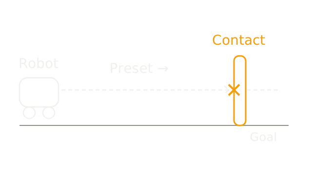
The dashed route is a preset command whose goal lies beyond an unexpected wall. The cross marks contact along that route. Open-loop execution does not use the resulting motion measurement to revise this command. Feedback offers a way to detect a change; it cannot guarantee a collision-free outcome.

2. Close The Loop

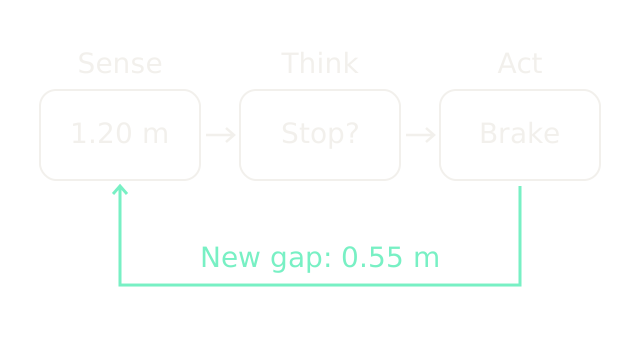
Sense supplies evidence, think estimates state and chooses a command, and act changes motion through physical forces. The bottom route returns a new range measurement after braking. This is the closed-loop structure described in Modern Robotics, Control System Overview. Our simplified triad groups estimation, planning and control; real robots can run these processes concurrently with different update rates.

3. Measure From The Front

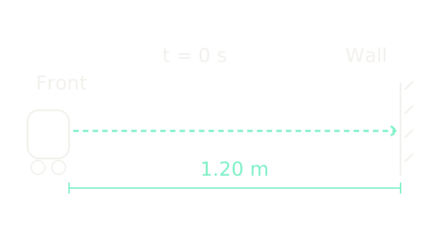
At time zero the front reference point has clearance 1.20 m and speed 1.0 m/s. The distance bracket begins at that front point, not the wheel centre. Spatial frames 3, 4 and 6 use 400 drawing units per metre. We assume exact, timestamped range and a stationary wall. Actual sampling adds waiting time; here the stated delay starts at the sample timestamp and includes all time until braking begins.

4. Account For Delay

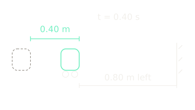
The dashed body is the old position and the solid body is the new position on the same scale. During a 0.40 s sensing-to-braking delay, constant speed gives travel $v\Delta t=1.0\times0.40=0.40$ m. The remaining gap is $1.20-0.40=0.80$ m. A correct decision based on the old range must account for this motion.

5. Braking Takes Distance

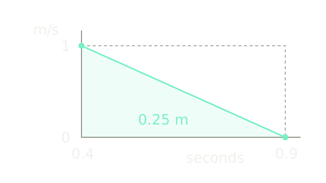
This view changes from position to velocity versus time. Braking starts at 0.40 s. Assume the brakes immediately produce a constant deceleration magnitude of 2.0 m/s² until rest. Speed reaches zero after $1.0/2.0=0.50$ s, at absolute time 0.90 s. The triangular area under the velocity trace is displacement:

$$d_{\mathrm{brake}}=\tfrac12(0.50)(1.0)=0.25\text{ m}=\frac{v^2}{2a}.$$

This idealization omits brake ramp-up, traction limits and wheel slip.

6. Add Both Costs

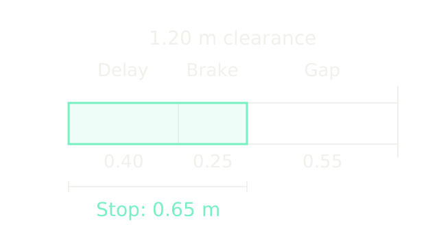
The contiguous segments divide the original 1.20 m gap. Delay uses 0.40 m, braking uses 0.25 m, and the last 0.55 m remains. Total stopping travel is $0.40+0.25=0.65$ m. The mint outline covers the first two segments; their widths preserve the same 400-unit-per-metre scale. Remaining clearance is a result of these assumptions, not a certified safety margin.

7. Use Different Update Rates

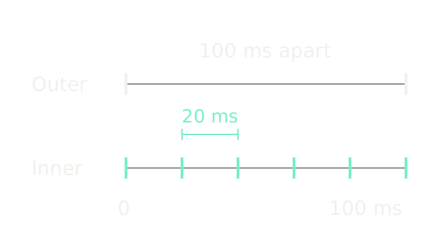
The aligned rows share one time axis. This illustrative outer loop updates every 100 ms (10 Hz); the inner loop updates every 20 ms (50 Hz), giving five inner intervals per outer interval. These are chosen teaching rates, not recommended hardware settings. An actuator loop can regulate current while a higher loop tracks motion or revises a route. The textbook's nested amplifier and motion loops motivate the structure; rates depend on dynamics, sensors and compute.

8. Detect A Disturbance

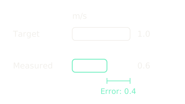
This comparison introduces a separate speed-control example. A load or slope lowers measured speed to 0.6 m/s while the target stays 1.0 m/s. Equal-scale bar lengths expose error $e_v=1.0-0.6=0.4$ m/s. The controller may request more drive, subject to its control law and torque limits. Error alone does not determine the required torque or recovery time; no such recovery claim is assumed here.

9. Stale Feedback Can Overshoot

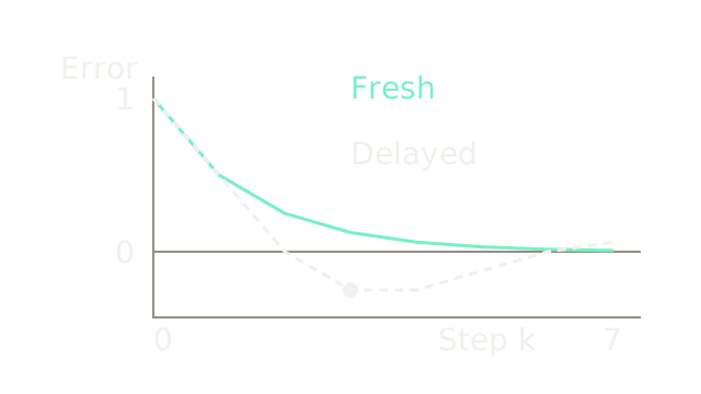
This unitless discrete model isolates delay rather than predicting the earlier vehicle. Let $x_{k+1}=x_k+u_k$, target $r=0$, and error $e_k=r-x_k$. With gain 0.5, fresh control $u_k=0.5e_k$ gives $e_{k+1}=0.5e_k$: from 1, errors are 0.5, 0.25, 0.125 and so on.

A one-step stale command $u_k=0.5e_{k-1}$ instead gives $e_{k+1}=e_k-0.5e_{k-1}$. Starting with $e_{-1}=e_0=1$, the plotted values are 1, 0.5, 0, −0.25, −0.25, −0.125, 0, 0.0625. The dashed trace crosses zero while the fresh trace approaches it from above. This case oscillates with decreasing amplitude; it does not demonstrate divergence. Fresh feedback also does not universally prevent overshoot: plant dynamics and gain matter.

10. Where It Breaks

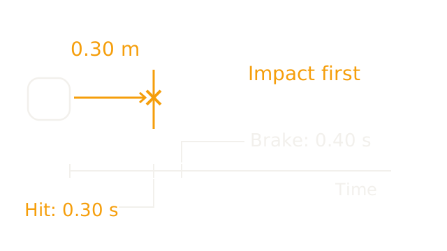
Return to the 1.0 m/s vehicle and 0.40 s delay, but change the initial wall clearance to 0.30 m. Contact occurs after $0.30/1.0=0.30$ s, before the braking command at 0.40 s. The spatial contact and event ruler are separate views, aligned because speed is one metre per second. Nothing shows the robot traveling through the wall.

Late feedback cannot recover already-lost stopping distance. Even obstacles beyond the delay travel can still be too close once braking distance is included. Slower speed, earlier detection and faster protective reactions can change the budget; this simplified model proves no universal safe operating distance.

The Quick Version

• A fixed command can fail when the world changes.
• Feedback connects a physical action to a fresh measurement.
• Range needs a timestamp and a stated reference point.
• Delay consumes distance before braking starts.
• Physical braking takes additional distance.
• Add delay travel and braking travel before judging clearance.
• Inner loops can update between outer-loop decisions.
• Speed error alone cannot determine recovery torque or time.
• Stale feedback can produce overshoot even in a converging system.
• A correct command can arrive after contact.