How Robots Sense

Robots estimate physical state from sensor measurements and a model of what those measurements mean. Wheel rotation can suggest motion even when a wheel slips; external observations can challenge that estimate. All values below are synthetic examples, not sensor specifications or measured performance.

1. Signals Need A Model

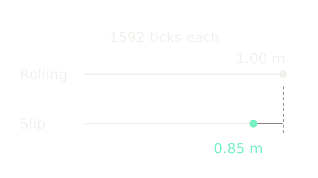
Both cases produce the same encoder count. Pure rolling gives about 1.00 m of chassis travel; the slipping case gives about 0.85 m. The rails share a scale, so the difference is physical motion rather than an altered drawing scale. An encoder measures rotation, a proprioceptive quantity internal to the robot. Inferring position requires assumptions about wheel radius, contact and heading.

2. Count Wheel Rotation

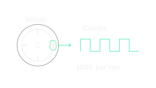
An optical encoder detects changes as a patterned disk rotates. The four drawn marks and pulse excerpt are schematic, not the actual number of slots. Assume wheel radius 0.10 m and 1,000 effective decoded counts per revolution. Count conventions depend on the encoder and decoding method.

One count corresponds to circumference travel $2\pi(0.10)/1000=0.0006283185$ m, about 0.628 mm. Therefore 1,592 counts give 1.0002831 m, which rounds to 1.00 m; it is not exactly one metre. This estimates wheel circumference travel, not necessarily body translation.

3. Sum Motion Increments

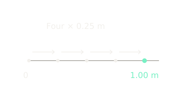
Four increments of 398 counts each imply approximately 0.2500708 m per increment and 1.0002831 m total. The picture rounds these to four 0.25 m steps on a common position ruler. Starting from a known position, one-dimensional dead reckoning sums them: $x_k=x_{k-1}+\Delta s_k$. In a turning robot, heading must also be integrated or measured. WPILib's odometry documentation describes combining wheel distances with heading and warns that the estimate can drift.

4. Expose Wheel Slip

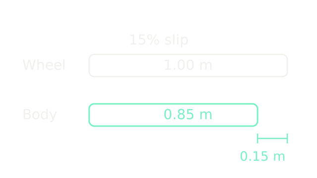
Define slip fraction here as $s=1-d_{\mathrm{body}}/d_{\mathrm{wheel}}$. At s = 0.15, body travel is $0.85\times1.0002831=0.8502406$ m and the difference is 0.1500425 m. Bars show the rounded values 1.00, 0.85 and 0.15 m. Odometry alone cannot identify this unobserved discrepancy. It is not permanently unrecoverable: independent observations can constrain accumulated error.

5. Observe An External Reference

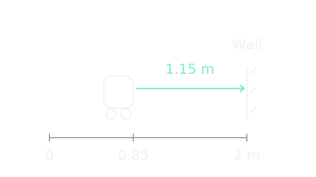
For the next idealized calculation, take the rounded values as exact model inputs. A wall is known to be at x = 2.00 m and the sensor measures a forward range of 1.15 m. With known alignment and sensor reference point, inferred sensor position is $2.00-1.15=0.85$ m. The range ray and absolute ruler share a 200-unit-per-metre spatial scale.

Pulsed time-of-flight LiDAR relates range to half the light round-trip distance, as described in SICK's LiDAR guide. A wall range alone does not determine full 3D pose. Wall identity, calibration, orientation and measurement error still matter.

6. Weight The Evidence

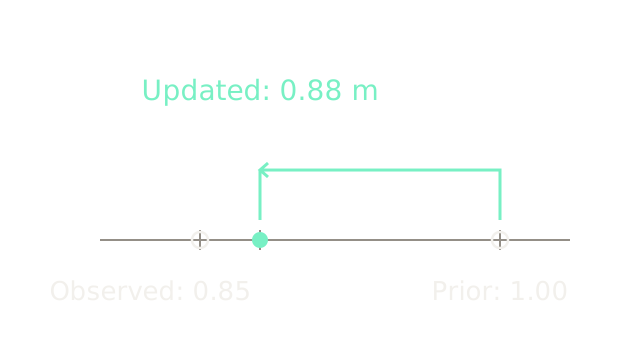
This number line deliberately zooms into position, using 2,000 drawing units per metre. A prior position estimate of 1.00 m has variance P = 0.01 m². Treat the independent, unbiased external position observation 0.85 m as having variance R = 0.0025 m². A scalar Kalman-style update gives:

$$K=\frac{P}{P+R}=0.8,\qquad \hat x^+=1.00+0.8(0.85-1.00)=0.88\text{ m}.$$

The arrow moves 80% of the way toward the observation. Updated variance is $(1-K)P=0.002$ m² under this model; uncertainty remains. Timestamp alignment, bias and correlated errors can invalidate the assumptions. WPILib pose estimators illustrate combining encoder and gyro updates with timestamped external pose evidence. Fusion can reduce drift; it does not universally eliminate it, and multiple sensors are not mandatory for every task.

7. Integrating Bias Twice

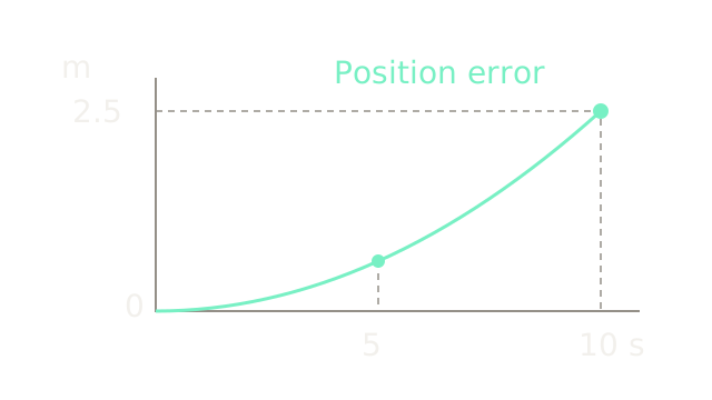
This separate inertial example assumes exact attitude and gravity removal, zero initial position/velocity errors, and an uncorrected constant horizontal accelerometer bias b = 0.05 m/s². Integrating bias once gives velocity error bt; integrating again gives position error $bt^2/2$. At 5 s it is 0.625 m; at 10 s it is 2.50 m. The exact quadratic curve uses common time and error axes.

An IMU measures angular rate and specific force; it does not directly measure global position. VectorNav's inertial sensor introduction discusses sensor types and bias stability. Real inertial errors can also involve attitude, gravity projection, noise and varying bias; this simple parabola isolates only one cause.

8. Infer Depth From Disparity

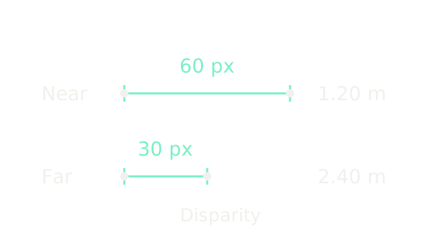
These are pixel-displacement rulers, not physical camera baselines. For a calibrated, rectified stereo pair, disparity is the horizontal separation of corresponding image locations after principal-point alignment. With focal length f = 600 pixels and camera baseline B = 0.12 m, $Z=fB/d$: 60 pixels gives 1.20 m depth, while 30 pixels gives 2.40 m. The rulers share four drawing units per pixel.

OpenCV's stereo depth tutorial explains this inverse relationship. It requires correct correspondence and calibration. Small disparity makes depth especially sensitive to pixel errors; occlusion and textureless surfaces may prevent a valid match.

9. Keep Measurement Uncertainty

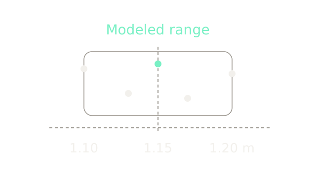
The five deliberately chosen readings are 1.10, 1.13, 1.15, 1.17 and 1.20 m around a modeled range of 1.15 m. Horizontal position carries range; vertical separation merely prevents the dots overlapping. The outline groups the illustrated spread and is not a confidence interval.

An additive zero-mean Gaussian model can be useful when its assumptions fit the sensor and operating conditions. These five synthetic points do not establish a distribution or a 68% coverage claim. Outliers, bias and missing returns require different handling from ordinary random scatter.

10. Where It Breaks

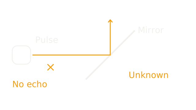
An ideal mirror tilted 45° redirects the incoming horizontal pulse upward, away from the receiver. The crossed return cue and “Unknown” label distinguish absent evidence from a measured long range. The drawn reflection obeys equal incidence and reflection angles.

Real glass can transmit, reflect or generate multiple returns depending on material, angle and settings; this is a simplified specular example. SICK's guide describes surface-dependent returns and glass limitations. Missing or invalid returns must not automatically become “free space.” Whether a robot stops, seeks another observation or proceeds depends on its sensor semantics and control policy; collision is not an inevitable sensor behavior.

The Quick Version

• Sensor readings require a model to infer physical state.
• Encoder counts describe rotation and require a decoding convention.
• Dead reckoning accumulates estimated increments.
• Slip separates wheel travel from chassis travel.
• Known external geometry can constrain accumulated position error.
• Weighted fusion retains uncertainty and depends on assumptions.
• Constant uncorrected acceleration bias yields quadratic position error here.
• Rectified stereo depth is inversely proportional to valid disparity.
• Gaussian noise is a model to check, not a universal fact.
• Missing laser returns do not prove free space.