Core ML

Autoencoders

Force data through a layer too narrow to hold it, then ask for the original back. Whatever survives the squeeze is the structure the data actually has.

An encoder squeezes the input down to a narrow code and a decoder rebuilds the input from it, so the loss compares the output with the input and needs no labels at all

Why Does This Exist?

A camera above a kiln photographs every ceramic floor tile coming off the line. Sixty-four pixels square, greyscale, 200,000 photos a week, none of them labelled. An inspector tagged 400 as cracked or fine, months ago, and that's your entire supervised dataset.

So 4096 numbers describe a tile. But tiles aren't 4096 different things. Same glaze, same grout spacing, same camera height — what varies is brightness, a little rotation, speckle density, and whether there's a crack. A dozen quantities; 4084 dimensions along for the ride.

An encoder here is nothing exotic: a stack of layers mapping numbers to numbers, a multi-layer perceptron. And dropping dimensions is already solved — PCA finds the flat subspace keeping the most variance and projects onto it.

Here's where flat runs out. Rotate a tile two degrees and every pixel changes, along a curve through pixel space, not a straight line. A flat subspace spends dimensions approximating that bend. You wanted the curve.

Think of It Like This

The card through the hatch

Two draughtsmen, a wall between them, one narrow slot. The first looks at a tile and writes 32 numbers on a card. The second, who never sees the tile, redraws it from the card alone. Score how close the redrawing comes, and repeat on this factory's tiles for a month.

They'll invent a shorthand. Number 3 becomes grout offset, number 11 becomes speckle density, because there's room for nothing else. Nobody handed them that vocabulary — the scoring produced it.

Two things follow, and both matter later. Widen the slot to a 4096-number card and they stop inventing anything: the first copies the pixels across, the score is perfect, the shorthand is gone. And if you invent 32 numbers yourself and post the card through, the second draughtsman draws something — it just isn't a tile.

How It Actually Works

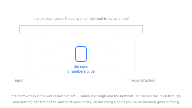
Two halves with a pinch in the middle. The encoder $f$ maps 4096 pixels down to a code $z$ of 32 numbers. The decoder $g$ maps $z$ back out to 4096. Training minimises how far the round trip lands from where it started:

\mathcal{L} = \frac{1}{n}\sum_{i=1}^{n} \big\lVert x_i - g(f(x_i)) \big\rVert^2

$x_i$ is one tile photo, $g(f(x_i))$ is the network's attempt at rebuilding it, and the bars mean squared difference summed over all 4096 pixels. Look at what isn't there: a label. The target is the input, which is what makes this self-supervised learning.

The bottleneck does the work

Thirty-two isn't a knob you tune for accuracy. It's the constraint that makes learning happen. With 4096 slots the cheapest solution is a copy, and a copy teaches nothing. With 32, every slot has to earn its place. Glaze brightness earns it. Pixel (17, 40) does not.

Where PCA ends and this starts

The relationship is exact, not a family resemblance. Make both halves single matrices with no activation, keep squared-error loss, and the optimum spans the same subspace as the top principal components. Same subspace, not the same axes — nothing in that loss asks for orthogonal or ordered directions.

So a linear autoencoder buys nothing over PCA except a slower way to compute it. The payoff arrives with the nonlinearities: the decoder traces a curved surface through pixel space instead of a flat slice, so two degrees of rotation becomes a short move along that surface. That surface is the latent manifold, and following it is the only reason to reach for a network.

Variants, and the hole none of them fill

Denoising is the one to reach for first. Knock out 30% of the input pixels at random and ask for the clean tile back. Copying is now actively wrong, so the network has to infer missing grout lines from the surrounding ones. Sparse autoencoders go the other way: keep the code wide, penalise how many units switch on, let activity be the limit instead of width. Both block the lazy path — and a roomy bottleneck really does let a network approximate the identity function, reconstruct beautifully, and teach nothing.

Now the limit the next page exists to fix. That loss says nothing about the space between codes. It scores 200,000 round trips and never asks what sits between two of them, so codes land wherever training put them and decoding a point you didn't encode gives mush. You can't sample either — you don't know what distribution the codes follow. Compression model, not a generative one. (Discrete-latent variants sidestep that by fitting a separate model over code sequences, the route to autoregressive generation.)

Show Me the Code

Fit a linear autoencoder by gradient descent, then take the principal angles between its encoder subspace and the top two principal components. Cosines near 1 mean the same subspace.

1import numpy as np2
3def fit_linear_autoencoder(x: np.ndarray, width: int, steps: int = 40_000) -> np.ndarray:4    rng = np.random.default_rng(0)5    enc = rng.normal(0.0, 0.1, (x.shape[1], width))6    dec = rng.normal(0.0, 0.1, (width, x.shape[1]))7    for _ in range(steps):  # no activation anywhere, so this is the linear case8        err = x @ enc @ dec - x  # squared error against the input itself9        enc -= 2e-2 * (x.T @ err @ dec.T) / len(x)10        dec -= 2e-2 * ((x @ enc).T @ err) / len(x)11    return enc12
13rng = np.random.default_rng(1)14tilt = rng.normal(0.0, 1.0, (2, 6))  # 500 points on a 2-D plane sitting inside 6-D15x = rng.normal(0.0, 1.0, (500, 2)) @ tilt + rng.normal(0.0, 0.05, (500, 6))16x -= x.mean(axis=0)17pca = np.linalg.svd(x, full_matrices=False)[2][:2]18overlap = np.linalg.svd(np.linalg.qr(fit_linear_autoencoder(x, 2))[0].T @ pca.T)[1]19print(np.round(overlap, 4))  # -> [0.9999 0.9998]

Two matrices found the plane PCA gets in closed form. Add a nonlinearity and that guarantee is gone, which is the point.

Watch Out For

A bottleneck wide enough to cheat through

Reconstruction error drops to almost nothing, so you ship it. Then the defect classifier trained on those 32 numbers performs like it's reading noise. The bottleneck had room to pass the input through nearly unchanged, so the code is a lightly scrambled copy of the pixels.

Reconstruction error can't catch it — that's what a cheating network optimises. Two things can. Check whether the code's dimensions carry independent information rather than a few dominating, and narrow the bottleneck on purpose: if downstream accuracy goes up when you cut 64 numbers to 16, the wide version was passing pixels.

Treating the latent space as something you can sample

Someone interpolates between two tile codes to make training examples, or draws 32 Gaussian numbers and decodes them. Out come smears and grey fog. The instinct is that the model undertrained.

It didn't. Nothing in the loss constrained the region between two encoded points, so a decoder asked about it returns garbage with full confidence. Test it: encode two real tiles, decode ten points along the line between their codes, look. If the midpoints aren't plausible tiles, closing those holes is what a variational autoencoder is for.

The Quick Version

An encoder squeezes the input to a short code, a decoder rebuilds it, and the loss is reconstruction error against the input. No labels.
The bottleneck is the mechanism. Too wide and the network learns the identity function and teaches you nothing.
Linear layers plus squared error span the same subspace as PCA, exactly. Nonlinearity earns its keep on curved structure.
Denoising asks for the clean version of a corrupted input. Sparse penalises activations instead of narrowing the layer.
Nothing structures the latent space, so unvisited points decode to nothing and sampling has no basis.