Core ML

Bias–Variance Tradeoff

Error splits into three parts: a wrong-shaped model, a jumpy one, and noise you can never fix. Only the first two are yours to trade against each other.

As model complexity rises, the bias term falls and the variance term climbs, so their sum is a U-shaped curve whose lowest point is the complexity worth shipping

Why Does This Exist?

Your model scores 0.98 on the data you trained it on and 0.71 on next month's data. Something ate twenty-seven points, and until you can name what, you're just guessing: more data, a bigger model, a smaller model, more features, fewer features.

This decomposition is the naming scheme. That gap has exactly three sources, two of them respond to opposite treatments, and the third responds to nothing. Treat the wrong one and you'll spend a week making the model measurably worse.

You're predicting a city's peak electricity demand from the day's high temperature. Demand climbs on freezing days because of heating and on hot days because of air conditioning, so the truth is roughly a U. You have fourteen days of history — fourteen points, each carrying real noise, because demand also depends on whether it was a weekday, whether the smelter was running, and a hundred things nobody wrote down.

Expected error is the average error across many reruns of the whole exercise: fresh fourteen days, refit, measure, repeat. It describes the procedure, not one fitted model. Variance is the ordinary statistical kind — see expectation, variance and covariance.

Think of It Like This

Three ways a bathroom scale can be wrong

Your scale reads 3 kg heavy. Every single time. Step on it ten times and you get ten identical wrong answers, so averaging more readings buys you nothing. That's bias: an offset baked into the instrument.

Swap it for a scale that reads 71, 78, 74, 80, 73. Average those and you land almost exactly on the truth. Any single reading is useless. That's variance: no systematic offset, but you can't trust one measurement, and one measurement is all production ever gives you.

Then there's the kilogram or so that genuinely moves across a day: water, a different hour. No scale removes it. That's irreducible noise, and it sets the floor.

How It Actually Works

Fix one input — say a 32 °C day. Ask what the expected squared error of your fitting procedure is at that temperature. It splits, exactly, into three terms:

\mathbb{E}\big[(y - \hat{f}(x))^2\big] = \big(\mathbb{E}[\hat{f}(x)] - f(x)\big)^2 + \operatorname{Var}\big[\hat{f}(x)\big] + \sigma^2

Read left to right. $f(x)$ is the truth. $\hat{f}(x)$ is what your procedure predicts — random, because the fourteen days you got were random. The first term is bias squared: how far the average prediction across all possible fourteen-day samples sits from the truth. The second is variance: how much your prediction jumps as the sample changes. The third, $\sigma^2$ , is the noise in demand itself.

That identity is not a heuristic. It's algebra, and it holds exactly for squared loss. Add and subtract $\mathbb{E}[\hat{f}(x)]$ inside the square, expand, and the cross-term integrates to zero.

Turning the complexity dial

Fit a straight line to the U. It's doomed: no straight line goes through a curve, so the average prediction is wrong at both ends and in the middle. High bias. But it's stubborn — swap in a different fourteen days and you get almost the same line. Low variance.

Now fit a degree-8 polynomial. It threads every point exactly, noise included, so its average prediction is close to the truth and bias is small. But change one of the fourteen days and the curve whips somewhere else. Enormous variance.

The parabola between them wins because the truth is a parabola. Right shape, few parameters.

Why the sum is a U

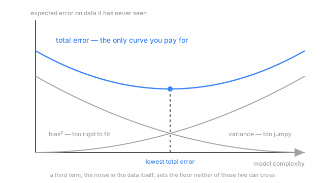
Bias falls as you add capacity. Variance rises. Their sum falls while bias dominates, bottoms out, then climbs while variance dominates — the U in the diagram, its minimum at the complexity worth shipping.

Two consequences people get backwards. The minimum is not at zero bias, so a model that fits its training data perfectly is virtually never the best one. And it moves right as you get more data, because data suppresses variance for free, freeing capacity to spend on bias. That's the honest reason "get more data" works so often.

The term that isn't a tradeoff

$\sigma^2$ never enters the tradeoff. It's the floor. If tomorrow's demand depends on a factory schedule you have no column for, no architecture recovers it.

So the useful question is never "what's my error". It's how far above the floor you are, and which movable term the gap is made of. Learning curves are how you find out: both errors high and close means bias, a wide persistent gap means variance.

Show Me the Code

The decomposition is measurable. Resample the fourteen days a few hundred times and watch the prediction at 7.5.

1import numpy as np2
3
4def truth(x: np.ndarray) -> np.ndarray:5    return 0.4 * (x - 5.0) ** 2  # peak demand is U-shaped in temperature6
7
8def decompose(degree: int, at: float = 7.5, trials: int = 400) -> tuple[float, float]:9    rng = np.random.default_rng(7)10    preds = np.empty(trials)11    for i in range(trials):  # 400 alternate universes of the same 14-day sample12        x = rng.uniform(0.0, 10.0, 14)13        y = truth(x) + rng.normal(0.0, 1.0, 14)  # the irreducible part14        preds[i] = np.polyval(np.polyfit(x, y, degree), at)15    return float(preds.mean() - truth(at)), float(preds.var())16
17
18for d in (1, 2, 8):19    bias, var = decompose(d)20    print(f"degree {d}: bias {bias:+6.2f}   variance {var:8.2f}")21    # -> degree 1: bias  +0.70   variance     1.7122    # -> degree 2: bias  -0.03   variance     0.1623    # -> degree 8: bias  -3.28   variance  2971.29

Degree 1 carries an offset it can never shed. Degree 2 matches the truth. Degree 8 pays 2971 in variance to touch every point — three orders of magnitude worse, from the same fourteen numbers.

Watch Out For

Reading the tradeoff off a single train/test split

Every term in that identity is an expectation over datasets. One split hands you one draw, so a validation score that beat the previous model by 0.3 points might be a better model, or might be which rows landed in which fold.

With fourteen points, or fourteen thousand, this is not a rounding concern. Repeated cross-validation with the spread reported beside the mean is the cheap fix, and it regularly reveals that two models you'd been ranking confidently are indistinguishable.

Treating the U as a law of nature

Keep adding capacity past the point where the model interpolates the training set and test error often falls again, sometimes below the first dip. That's double descent, it's reproducible, and it's why a 70-billion-parameter model isn't automatically drowning in variance.

The identity still holds — it's algebra. What breaks is the assumption that parameter count proxies the variance term. Heavily overparameterised, the optimiser's own preference for smooth solutions acts as regularisation, so capacity and effective capacity come apart. Use the decomposition to diagnose what your error is made of, not to predict it from a parameter count.

The Quick Version

Expected squared error splits exactly into bias², variance, and irreducible noise. Algebra, not analogy.
Bias is being consistently wrong. Variance is being unstable across samples. Noise never leaves.
Bias falls and variance rises with complexity, so total error is U-shaped and the best model never fits its training data perfectly.
More data moves the minimum toward higher complexity, because it suppresses variance for free.
Diagnose before treating. Both errors high and close means bias; a wide persistent gap means variance. Opposite fixes.
The clean three-way identity is a squared-loss result. For 0–1 loss the intuition survives, the algebra doesn't.