Gen AI

Compute-Optimal Training

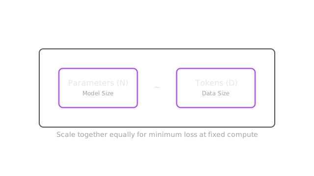
To get the smartest possible model for a fixed budget, parameter count and training data must be scaled equally; historically, models were too large and severely undertrained.

Why Does This Exist?

In the early days of large language models, the prevailing strategy was simply "bigger is better." Researchers poured their massive compute budgets into building models with staggering parameter counts (like GPT-3's 175 billion or Gopher's 280 billion), while keeping the amount of training data relatively flat. The result was a generation of bloated models that were immensely expensive to run in production, yet surprisingly fragile.

In 2022, DeepMind published the "Chinchilla" paper, which proved that this strategy was mathematically flawed. They demonstrated that to get the lowest possible error rate for a fixed amount of compute, you must scale the model size and the dataset size equally. The entire industry realized they had been building models that were too large and starved for data. Compute-optimal training is the mathematical framework that corrected this, dictating exactly how to balance parameters and tokens to extract the maximum intelligence per dollar.

Think of It Like This

Studying for an exam: Brain size vs. Reading material

Imagine you have exactly 100 hours to prepare for a medical exam. You can spend that budget in two ways:

You can spend 90 hours memorizing a tiny, 10-page pamphlet perfectly. (Small data, huge effort)
You can briefly skim an entire 10,000-page medical library once. (Huge data, small effort)

Neither is optimal. In the first scenario, you've over-studied a tiny amount of information; you lack the breadth to answer general questions. In the second, you've seen everything but absorbed nothing.

Compute-optimal training is finding the exact sweet spot: spending your 100 hours reading a moderately sized, 500-page textbook thoroughly. The Chinchilla laws dictate that if you are given 200 hours next time, you shouldn't just read the 500-page book twice as hard; you should read a 1,000-page book with the exact same level of effort.

How It Actually Works

The Chinchilla ratio

The core finding of compute-optimal training is often summarized as a simple ratio: for every single parameter in a model, you should train it on roughly 20 tokens of data.

If you have a budget to train a 10-billion parameter model, you should feed it 200 billion tokens. If you increase the model size by 10x to 100 billion parameters, you must also increase the data by 10x to 2 trillion tokens. Previous scaling laws incorrectly suggested that as compute increased, model size should grow much faster than data size. The Chinchilla paper proved that they must grow at roughly a 1:1 proportion.

The cost of ignoring the ratio

If you violate the compute-optimal ratio by building a model with too many parameters for your data budget (e.g., 280 billion parameters trained on only 300 billion tokens), you are wasting compute. The model will memorize the small dataset and fail to generalize. Worse, you are left with a bloated, 280-billion parameter monstrosity that costs a fortune in GPU RAM to host during inference.

If you violate the ratio in the other direction—training a tiny model on an endless ocean of data—the model simply lacks the neural capacity (the parameters) to absorb the complexity of the information, and its learning curve flatlines.

Pushing past compute-optimal for inference

Interestingly, modern labs often intentionally violate the Chinchilla ratio in one specific direction: they heavily overtrain small models. Llama 3 8B, for example, has 8 billion parameters but was trained on an astonishing 15 trillion tokens—massively exceeding the 20x ratio.

Why? Because the Chinchilla laws optimize for the cheapest training cost. But in the real world, a model is trained once and deployed millions of times. By spending extra compute during training to push a tiny 8B model to its absolute limits, Meta created a model that is incredibly cheap and fast to run during inference. It is not compute-optimal for training, but it is highly optimal for long-term deployment.

Show Me the Code

Calculating the compute-optimal allocation between parameters (N) and tokens (D) for a given compute budget (C) is straightforward algebra based on the Chinchilla paper's approximations.

The training compute in FLOPs is roughly $C \approx 6 \times N \times D$ . If we want $D \approx 20 \times N$ , we can solve for N.

1import math2
3def calculate_optimal_allocation(compute_flops: float) -> tuple[float, float]:4    """5    Given a total compute budget in FLOPs, calculates the optimal 6    model size (Parameters) and dataset size (Tokens).7    Uses the approximation C = 6 * N * D, where D = 20 * N.8    Therefore: C = 6 * N * (20 * N) = 120 * N^29    """10    # Solve for N: N^2 = C / 12011    optimal_parameters = math.sqrt(compute_flops / 120)12    13    # D is 20x the parameters14    optimal_tokens = 20 * optimal_parameters15    16    return optimal_parameters, optimal_tokens17
18budget = 1e21  # Example FLOP budget for a medium-scale run19
20params, tokens = calculate_optimal_allocation(budget)21
22print(f"Optimal Parameters: {params / 1e9:.1f} Billion")23print(f"Optimal Tokens:     {tokens / 1e9:.1f} Billion")24print(f"Ratio (Tokens/Params): {tokens / params:.1f}x")25
26# -> Optimal Parameters: 91.3 Billion27# -> Optimal Tokens:     1825.7 Billion28# -> Ratio (Tokens/Params): 20.0x

This math proves that for $10^{21}$ FLOPs, building a 90B model and training it on 1.8T tokens is mathematically superior to building a 175B model and starving it of data.

Watch Out For

Confusing compute-optimal with inference-optimal

As mentioned above, Chinchilla compute-optimal training strictly minimizes the FLOPs required during the training phase to reach a specific loss. It completely ignores the cost of running the model afterward. If you want a model that is cheap to host, you should deliberately overtrain a smaller model past the Chinchilla optimal point.

Treating the 20x ratio as a law of physics

The ~20x ratio of tokens to parameters is an empirical observation based on specific architectures and datasets from 2022. It is a highly useful rule of thumb, but it is not a fundamental constant of the universe. Variations in data quality, vocabulary size, and architectural efficiency can shift the optimal ratio higher or lower.

The Quick Version

Compute-optimal training dictates how to balance model size (parameters) and dataset size (tokens) to get the smartest model for a fixed compute budget.
The Chinchilla paper proved that early models were too large and severely undertrained; parameters and data must be scaled equally.
The general rule of thumb is that a model should be trained on roughly 20 tokens for every parameter it contains.
Many modern models are intentionally trained past this optimal point (overtrained) to keep the parameter count small, making them cheaper to deploy in production.