Math

Central Limit Theorem

Averages become bell-shaped no matter what they are averages of — which is the one fact that makes error bars, p-values and confidence intervals possible at all.

Averages turn bell-shaped no matter what they are averages of: a flat die-roll distribution becomes triangular by two rolls and near-normal by thirty, which is why standard errors work at all

Why Does This Exist?

Your accuracy metric is an average. So is your mean loss, your average latency, and every number on your evaluation dashboard. And every one of them was computed from a sample — this test set, this batch, this week's traffic — not from the truth.

So how far from the truth might it be? Without an answer to that, comparing 87% against 89% is guesswork. The central limit theorem is the answer, and it is remarkable how little it asks for: you do not need to know the distribution of your data. Whatever shape it has — skewed latency, binary correctness, heavy-tailed token counts — the average is approximately normal, and you can put a number on its spread.

Everything downstream depends on this. The $\sqrt{n}$ in every standard error, the 1.96 in every 95% interval, the normal approximation behind most tests. It is also the honest reason large test sets matter, and the reason the returns diminish the way they do.

Think of It Like This

Guessing the average height of a city

You want the average height of everyone in a city, and you can only measure a few people.

Measure one person and your estimate is whatever they happen to be. Land on a basketball player and you are badly wrong. The spread of possible answers is exactly the spread of human height.

Measure ten and average them. Now a single tall person is diluted by nine others, so your estimate cannot swing as far. To be badly wrong you would need most of your ten to be unusual in the same direction, which is much less likely.

Measure a thousand and the average is very stable. Extremes in both directions cancel out.

Two things happened. Your estimate got less variable, and the pattern of remaining error became bell-shaped — small errors common, large ones rare, symmetric in both directions — even though the underlying height distribution is not symmetric.

The catch is the rate. To halve your uncertainty you need four times the people, not twice. That is the $\sqrt{n}$ , and it is why the last percent of confidence is so expensive.

How It Actually Works

Take independent samples $X_1, \ldots, X_n$ from any distribution with mean $\mu$ and finite variance $\sigma^2$ . Their average $\bar X$ has:

E[\bar X] = \mu, \qquad \text{Var}(\bar X) = \frac{\sigma^2}{n}

In plain words: the average is centred on the truth, and its variance shrinks in proportion to $1/n$ . The first part is what "unbiased" means; the second is the useful part.

Taking the square root gives the standard error — the standard deviation of your estimate, not of your data:

\text{SE} = \frac{\sigma}{\sqrt{n}}

The central limit theorem adds the shape:

\bar X \;\dot\sim\; \mathcal{N}\!\left(\mu,\; \frac{\sigma^2}{n}\right) \quad \text{as } n \text{ grows}

In plain words: the sampling distribution of the average approaches a normal distribution, whatever the original data looked like. The convergence is in shape, and it holds for any distribution with finite variance.

Standard deviation is not standard error

This is the confusion worth eliminating early, because the two get swapped constantly in reported results.

Standard deviation $\sigma$ describes the data. More data does not change it — you just measure it better.
Standard error $\sigma/\sqrt{n}$ describes your estimate of the mean. More data shrinks it toward zero.

So "accuracy 87% ± 15%" is ambiguous and probably wrong: if 15% is the spread across folds that is a standard deviation, and if it is the uncertainty in the mean it should be divided by $\sqrt{n}$ . Error bars on a benchmark should be standard errors. Say which you used.

The law of large numbers is the weaker sibling

The law of large numbers says $\bar X \to \mu$ as $n \to \infty$ — the average converges to the truth. Useful, and it says nothing about how fast or in what pattern.

The CLT is the quantitative version: it gives the rate ( $1/\sqrt{n}$ ) and the shape (normal). That is what lets you compute an interval rather than merely trust that more data helps.

When it fails

Three conditions, and each has a real ML counterpart:

Finite variance. Heavy-tailed distributions with infinite variance break it outright. Rare in practice but not never — some latency and financial return distributions are close enough to cause trouble.
Independence. This is the one that actually bites. Correlated samples behave like a smaller effective sample, so your standard error is too small and your confidence is inflated. Time-series data, repeated measurements on the same user, and augmented copies of the same image all violate it.
Enough samples. " $n \ge 30$ " is a rule of thumb, not a theorem. Badly skewed data needs far more; for a proportion the usual guide is at least 10 expected successes and 10 expected failures, which matters for rare-event classification.

Worked example

A fair six-sided die. Its mean is $\mu = 3.5$ and its variance is:

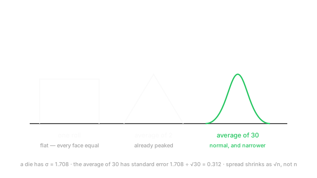
\sigma^2 = \frac{1}{6}\sum_{k=1}^{6}(k - 3.5)^2 = \frac{6.25 + 2.25 + 0.25 + 0.25 + 2.25 + 6.25}{6} = \frac{17.5}{6} \approx 2.9167

so $\sigma \approx 1.7078$ . The population is perfectly flat — nothing bell-shaped about it.

Now average 30 rolls. The mean of that average is still 3.5, and the standard error is:

\text{SE} = \frac{1.7078}{\sqrt{30}} = \frac{1.7078}{5.4772} \approx 0.3118

In plain words: the average of 30 rolls typically lands within about 0.31 of 3.5, and its distribution is close to normal despite the flat original. So roughly 95% of such averages fall in $3.5 \pm 1.96 \times 0.3118 = [2.89, 4.11]$ .

Watch the $\sqrt{n}$ cost. At $n = 30$ , SE is 0.312. To halve it to 0.156 you need $n = 120$ — four times the data. To reach 0.031, ten times smaller, you need $n = 3000$ , a hundredfold increase.

The same arithmetic on an accuracy metric: for a proportion, $\sigma = \sqrt{p(1-p)}$ , so at $p = 0.87$ and $n = 1000$ , $\text{SE} = \sqrt{0.87 \times 0.13 / 1000} \approx 0.0106$ . About one percentage point — which is exactly why a two-point gap between models is not obviously real.

Show Me the Code

1import numpy as np2
3rng = np.random.default_rng(0)4die = np.array([1, 2, 3, 4, 5, 6], dtype=float)5
6mu, sigma = die.mean(), die.std()                  # population, not a sample7print(mu, round(float(sigma), 4))                   # -> 3.5 1.70788
9n = 3010print(round(float(sigma / np.sqrt(n)), 4))          # -> 0.3118  predicted SE11
12# Simulate: 100,000 experiments, each averaging 30 rolls.13means = rng.choice(die, size=(100_000, n)).mean(axis=1)   # shape (100000,)14print(round(float(means.mean()), 3), round(float(means.std()), 4))  # -> 3.5 ~0.311815
16# Quadrupling n halves the SE — the sqrt(n) tax, not a linear one.17for k in (30, 120, 3000):18    print(k, round(float(sigma / np.sqrt(k)), 4))    # -> 0.3118, 0.1559, 0.031219
20# A proportion: accuracy 87% on 1000 examples.21p = 0.8722print(round(float(np.sqrt(p * (1 - p) / 1000)), 4)) # -> 0.0106  about 1 point

The simulated standard deviation of the averages matches the predicted 0.3118 — the theorem confirmed empirically, from a flat starting distribution.

Watch Out For

Computing a standard error on correlated samples

The independence assumption is the one that fails silently and most often, and the consequence is always in the dangerous direction: your uncertainty comes out too small, so you become confident about a difference that is not there.

The mechanism is that correlated observations carry less information than independent ones. With positive correlation, the effective sample size is smaller than $n$ — sometimes far smaller — so dividing by $\sqrt{n}$ overstates how much averaging you actually did.

Four common cases in ML. Time-series splits where adjacent points are highly correlated. Multiple rows per user, where 10,000 rows from 500 users is closer to $n = 500$ than $n = 10{,}000$ . Augmented data, where twenty crops of one image are one image. And cross-validation folds, which share training data by construction and are therefore not independent — the standard deviation across folds systematically understates the true variability.

Fixes that work: group your splits by the unit of independence (GroupKFold by user), compute an effective sample size when autocorrelation is present, or use a block bootstrap that resamples whole blocks rather than individual rows. The question to ask before dividing by $\sqrt{n}$ is always " $n$ what, exactly?" — and the honest answer is the count of independent units, not of rows.

Trusting the normal approximation on rare events

" $n \ge 30$ " fails badly for proportions when the event is rare, and rare-event classification is a large slice of applied ML.

The usual guide for a proportion is at least 10 expected successes and 10 expected failures. With $p = 0.001$ you need $n = 10{,}000$ just to expect 10 positives. Below that the sampling distribution is skewed and bounded at zero, so the symmetric normal interval is simply the wrong shape — and it will happily produce a lower bound below zero, which is a clear tell that the approximation has broken.

This is exactly the regime of fraud detection, medical screening, and safety classifiers. Report a 95% interval on a recall estimated from 8 positive cases using the normal formula and the interval is meaningless.

Use an interval built for proportions instead. The Wilson score interval is well behaved at small counts and never leaves $[0,1]$ ; the Clopper–Pearson interval is exact and conservative. Both are one call in statsmodels.stats.proportion. And for a metric with no formula at all — F1, AUC, a median — use the bootstrap, which makes no normality assumption.

The Quick Version

The average of a sample is centred on the truth, with variance $\sigma^2/n$ .
Standard error is $\sigma/\sqrt{n}$ : the spread of your estimate, not of your data.
The CLT says that average is approximately normal whatever the data's distribution, given finite variance.
Standard deviation describes the data and does not shrink with $n$ . Standard error describes the estimate and does.
Error bars on a benchmark should be standard errors. State which you reported.
The law of large numbers says the average converges; the CLT gives the rate and the shape.
Uncertainty falls as $\sqrt{n}$ : four times the data to halve it, a hundred times to divide it by ten.
Requires finite variance, independence, and enough samples. Independence is the one that breaks.
Correlated samples make the standard error too small. Ask " $n$ independent whats?"
For rare events use Wilson or Clopper–Pearson, not the normal approximation. Below 10 expected successes the normal interval is the wrong shape.