Math

Confidence Intervals

A range around an estimate, built by a recipe that lands on the truth most of the time — which is a promise about the recipe, not about the range you happen to be holding.

A ninety-five percent confidence interval is a promise about the procedure, not about any one interval: repeat the experiment and roughly one in twenty of the intervals you build will miss the true value entirely

Why Does This Exist?

Two models score 87% and 89% on your test set. Ship the second one?

The question is unanswerable from those numbers alone, and a confidence interval is what makes it answerable. With 1,000 test examples, 87% carries an interval of roughly ±2.1 points — so the two models' intervals overlap almost entirely, and the gap you are about to make a decision on is inside the noise.

This is the single most useful statistical habit in applied ML, and it is routinely skipped. Every leaderboard number, every A/B result, every "we improved recall by 1.5%" is a point estimate from a finite sample, and without a range it is impossible to tell a real improvement from a lucky draw.

There is also a definitional trap here that trips up almost everyone, including people who use intervals daily: a 95% confidence interval does not mean a 95% probability that the true value is inside it. What it does mean is worth getting exactly right.

Think of It Like This

A ring toss where you cannot see the peg

You are throwing rings at a peg in the dark. You cannot see the peg and you never find out whether you hit.

You know one thing about your technique: it lands over the peg 95 times out of 100. That is a property of your throwing, established over many attempts.

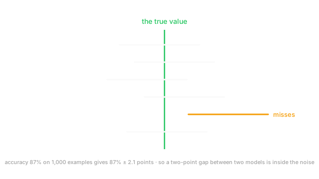
Now you throw one ring. Did it land over the peg? You have no idea. The 95% describes your technique, not this throw. This particular ring either encircles the peg or it does not — there is nothing probabilistic left about it once it has landed.

That is exactly what a confidence interval is. The recipe captures the true value 95% of the time across hypothetical repetitions. The specific interval you computed either contains it or does not, and you will never know which.

The diagram shows five rings that landed over the peg and one that missed, which is the honest picture. If you want to say "there is a 95% probability the value is in this interval", you are asking for a Bayesian credible interval — a different object requiring a prior.

How It Actually Works

The standard construction is an estimate plus or minus a multiple of its uncertainty:

\hat\theta \pm z \cdot \text{SE}

Three pieces. $\hat\theta$ is your estimate. $\text{SE} = \sigma/\sqrt{n}$ is the standard error, the spread of the estimate. And $z$ is a multiplier set by the confidence level you want — 1.96 for 95%, 2.576 for 99%, 1.645 for 90%.

The 1.96 comes from the normal distribution: 95% of a normal's mass lies within 1.96 standard deviations of its centre. So the whole construction leans on the central limit theorem making the estimate approximately normal.

For a proportion such as accuracy, $\sigma = \sqrt{p(1-p)}$ , giving:

\hat p \pm z\sqrt{\frac{\hat p(1 - \hat p)}{n}}

What the level actually promises

A 95% confidence interval means: if you repeated the whole experiment many times, 95% of the intervals you construct would contain the true value. The randomness is in the interval, not in the parameter.

Four things follow, and each one is a common error prevented:

You cannot say "95% probability the truth is in this interval." The truth is a fixed number; it is either in or out.
A wider interval is not a worse result — it is an honest one. Narrow intervals come from large $n$ , and faking them by assuming independence you do not have is the real failure.
Overlapping intervals do not prove no difference, and non-overlapping ones do not prove there is one. For comparing two estimates you want an interval on the difference, which is a different calculation.
The level is a choice, not a fact. 95% is convention, and the conventional choice is what makes multiple comparisons a problem.

The relationship to hypothesis testing

They are two views of one calculation. A 95% interval excludes a value exactly when a two-sided test against that value would reject at $p < 0.05$ .

So the interval strictly dominates in usefulness: it tells you whether the result is distinguishable from a baseline and how large the effect plausibly is. A p-value gives you only the first half. Prefer intervals for reporting.

When the standard formula is wrong

The $\hat p \pm z \cdot \text{SE}$ form (the Wald interval) is the one everybody writes and it misbehaves in two identifiable regimes:

Near 0 or 1. At $\hat p = 0.99$ with $n = 100$ , the interval extends past 1.0, which is impossible for a proportion. At $\hat p = 0$ it collapses to zero width, claiming certainty from having seen no events.
Small counts. Below roughly 10 expected successes and 10 expected failures the sampling distribution is skewed, so a symmetric interval is the wrong shape.

The Wilson score interval fixes both — it stays inside $[0,1]$ and behaves at small counts. Clopper–Pearson is exact and conservative. Both are one call in statsmodels. And for any statistic with no closed-form standard error — F1, AUC, a median — use the bootstrap.

Worked example

A model scores 87% accuracy on 1,000 test examples. What is the 95% interval?

The standard error for a proportion:

\text{SE} = \sqrt{\frac{0.87 \times 0.13}{1000}} = \sqrt{\frac{0.1131}{1000}} = \sqrt{0.0001131} \approx 0.01064

The margin of error is $1.96 \times 0.01064 \approx 0.02085$ , so:

\text{CI}_{95\%} = 0.87 \pm 0.0209 = [0.849,\; 0.891]

In plain words: about 87% give or take 2.1 points.

Now the decision the page opened with. The second model's 89% has essentially the same standard error, giving $[0.869, 0.911]$ . The intervals overlap across the range 0.869 to 0.891 — a wide shared region. So the data does not distinguish the two models, and the honest report is "89% ± 2.1 versus 87% ± 2.1, not distinguishable at this sample size".

How much data would settle it? To resolve a 2-point difference you want a margin of error well under 2 points, say 0.5. Since the margin scales as $1/\sqrt{n}$ , shrinking it from 2.1 to 0.5 — a factor of 4.2 — needs $4.2^2 \approx 17.6$ times the data, so roughly 17,600 test examples. That is the real cost of the claim, and it is the kind of number worth knowing before promising a result.

Show Me the Code

1import numpy as np2from statsmodels.stats.proportion import proportion_confint3
4
5def wald_ci(p: float, n: int, z: float = 1.96) -> tuple[float, float]:6    se = np.sqrt(p * (1 - p) / n)7    return p - z * se, p + z * se8
9
10print(round(float(np.sqrt(0.87 * 0.13 / 1000)), 5))    # -> 0.01064  standard error11print(np.round(wald_ci(0.87, 1000), 4))                 # -> [0.8491 0.8909]12print(np.round(wald_ci(0.89, 1000), 4))                 # -> [0.8706 0.9094]  overlaps13
14# Wald breaks near the boundary; Wilson does not.15print(np.round(wald_ci(0.99, 100), 4))                  # -> [0.9705 1.0095]  above 116print(np.round(proportion_confint(99, 100, method="wilson"), 4))   # -> [0.9462 0.9982]17print(np.round(proportion_confint(0, 30, method="wilson"), 4))     # -> [0. 0.1128]18
19# n needed to shrink the margin from 2.1 points to 0.5.20print(int(1000 * (0.0209 / 0.005) ** 2))                # -> 17472  ~17.5x the data

The 0.01064 and the interval [0.849, 0.891] match the hand calculation. The Wald interval reaching 1.0095 is the boundary failure, and Wilson's [0, 0.1128] from zero successes is the sensible answer where Wald would claim [0, 0].

Watch Out For

Comparing two estimates by checking whether their intervals overlap

This is the most common misuse, and it errs in both directions.

Non-overlapping intervals are conservative evidence of a difference — by the time two 95% intervals separate, the difference is significant at well beyond $p = 0.05$ . So you will miss real differences.

Overlapping intervals are not evidence of no difference. Two intervals can overlap substantially while the difference between the estimates is statistically significant, because the standard error of a difference is not the sum of the individual standard errors. For independent estimates it is $\sqrt{\text{SE}_1^2 + \text{SE}_2^2}$ , which is smaller than $\text{SE}_1 + \text{SE}_2$ .

The correct move is to build an interval on the difference itself. And when the two models were evaluated on the same test set — which is the usual case — they are not independent, and a paired test is both correct and much more powerful. McNemar's test for classification compares only the examples where the two models disagree, which is where all the information about the difference lives. Using it can resolve differences that unpaired analysis cannot.

Computing an interval on the data you selected with

If you use a validation set to pick the best of many configurations and then report a confidence interval on that winner's validation score, the interval is biased optimistically and the bias can be larger than the interval's own width.

The mechanism is selection. Try 50 configurations and the best validation score is partly genuine quality and partly the luckiest noise draw. The formula for the interval has no knowledge that a maximum was taken over 50 attempts, so it centres on an inflated estimate and reports a range that does not cover the truth anywhere near 95% of the time. This is the same arithmetic as multiple comparisons, showing up as bias instead of as a false positive.

It is why leaderboard scores drift upward over time while real-world performance does not, and it is why a model that looked 2 points better in a sweep so often lands flat in production.

The fix is a held-out test set touched exactly once, after all selection is complete. Report the interval from that. If you cannot afford a third split, nested cross-validation gives an approximately unbiased estimate at higher cost. And when you report a tuned number, say how many configurations were tried — that count is part of the result.

The Quick Version

$\hat\theta \pm z \cdot \text{SE}$ , with $z = 1.96$ for 95%, 2.576 for 99%, 1.645 for 90%.
For a proportion, $\text{SE} = \sqrt{\hat p(1-\hat p)/n}$ .
The level is a property of the procedure: 95% of intervals built this way contain the truth. Not a probability about the one you have.
For a probability statement about the parameter you need a Bayesian credible interval, which requires a prior.
A wider interval is a more honest one, not a worse result.
Intervals and tests are the same calculation. The interval also tells you the effect size, so prefer it for reporting.
87% on 1,000 examples is ±2.1 points, which is why a 2-point model gap is not a result.
Resolving that gap needs roughly 17,500 examples — the $\sqrt{n}$ tax made concrete.
Wald intervals break near 0 and 1 and at small counts. Use Wilson or Clopper–Pearson; bootstrap for statistics with no formula.
Do not compare by overlap — build an interval on the difference, and pair it when both models saw the same test set.
Never report an interval on the score you selected with. Use a held-out set touched once.