Math

Bootstrap and Resampling

Instead of deriving a formula for how uncertain your estimate is, resample your own data thousands of times and watch how much the answer moves.

Rather than deriving a formula, the bootstrap resamples the data you already have thousands of times and reads the spread of the answers straight off the results

Why Does This Exist?

There is a standard error formula for a mean and for a proportion. There is no usable one for the metrics you actually report.

F1 score, AUC, precision at $k$ , a median latency, the correlation between two model outputs, the gap between two models' F1 — none of these have a clean closed-form standard error, and several have none at all. So the question "is this F1 improvement real?" has no formula to answer it.

The bootstrap answers it anyway, and it does so with one idea: your sample is the best available stand-in for the population, so resampling from it imitates drawing fresh samples. No distributional assumption, no derivation, works on any statistic you can compute. Efron's insight in 1979, and it became practical the moment computers were cheap.

You already use it without noticing. Random forests are bootstrap aggregation. Their out-of-bag error estimate is a direct consequence of the arithmetic on this page.

Think of It Like This

A jar of marbles you are not allowed to refill

You want to know how much a survey result would wobble if you ran it again. The honest approach is to run it again — many times — and watch the spread. You cannot: you have one sample and no budget for more.

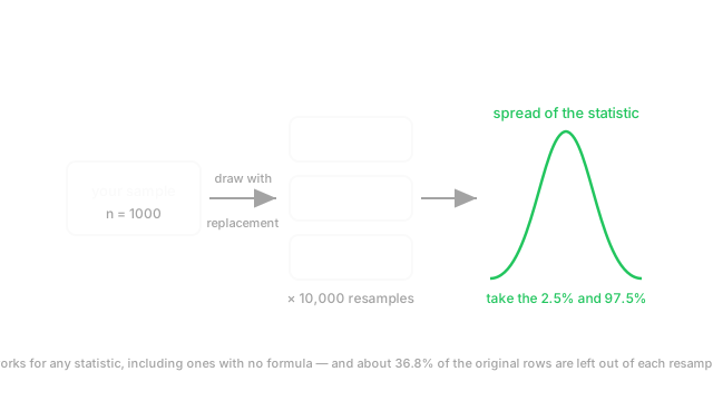
So do this instead. Put your 1,000 responses in a jar. Draw one, write it down, put it back, and repeat 1,000 times. You now have a new sample of 1,000 built entirely from what you already had. Some responses appear twice or three times, and roughly a third do not appear at all.

Compute your statistic on that fake sample. Then build another, and another, ten thousand times. You end up with ten thousand values of the statistic, and their spread tells you how much it wobbles.

The replacement is the crucial detail. Without it, every draw returns the identical original sample and you learn nothing. With it, each resample is a plausible alternative version of the data you might have collected — and the variation across those versions is the sampling variation you were trying to measure.

How It Actually Works

Four steps:

From your sample of size $n$ , draw $n$ observations with replacement.
Compute your statistic on that resample.
Repeat $B$ times, typically 2,000 for a standard error and 10,000 for an interval.
The spread of the $B$ values is the sampling distribution of your statistic.

From those values you read off what you need. The standard deviation of them is the standard error. And the percentile interval — the 2.5th and 97.5th percentiles for 95% coverage — is the simplest confidence interval.

The reason this works is the plug-in principle: the true sampling distribution comes from drawing samples from the population, and drawing from your sample approximates it. As $n$ grows, your sample resembles the population more closely and the approximation improves.

The 36.8% that gets left out

Here is the fact that makes the bootstrap more than a trick. The chance a specific observation is missed by one resample is:

\left(1 - \frac{1}{n}\right)^{n} \;\xrightarrow{\;n \to \infty\;}\; \frac{1}{e} \approx 0.368

In plain words: about 37% of your rows are absent from any given resample, and about 63% appear at least once.

That 37% is free held-out data. Train on the resample, evaluate on the rows it omitted, and you have an honest estimate with no separate validation split. This is exactly the out-of-bag error in a random forest — every tree is trained on a bootstrap resample and scored on the third of the data it never saw. Bagging's variance reduction comes from the same source.

Which interval

Percentile — take the 2.5th and 97.5th percentiles of the bootstrap values. Simple, and good enough for most reporting.
Basic / reverse percentile — reflects the percentiles around the original estimate. Better when the statistic is biased.
BCa (bias-corrected and accelerated) — corrects for both bias and skewness. The best general choice, and what scipy.stats.bootstrap uses by default.

Use BCa when it is available and the statistic is skewed or bounded. Percentile is fine when you just need a defensible range.

Permutation tests are the same family

For a hypothesis test rather than an interval, permute instead of resample. To test whether two models differ, pool their per-example results, repeatedly shuffle the labels between the two groups, and see how often chance produces a gap as large as the one you observed. That fraction is your p-value.

No distributional assumption, and it works on any statistic. When you cannot find the right test, a permutation test is almost always available and almost always defensible.

Where it breaks

The bootstrap is not universal, and the failures are specific:

Extremes. The maximum, the minimum, and very high quantiles are estimated badly, because a resample can never contain a value larger than the largest you observed.
Dependence. Resampling individual rows destroys time-series correlation and within-group structure. Use a block bootstrap for time series and resample whole groups for clustered data.
Tiny samples. With $n = 10$ the sample is a poor stand-in for the population, so the interval is unreliable however many resamples you draw.
Heavy tails. Convergence is slow when variance is huge or infinite.

Worked example

The out-of-bag arithmetic, exactly.

For $n = 5$ , the chance a given row is missed by all five draws is:

\left(\frac{4}{5}\right)^{5} = \frac{1024}{3125} = 0.32768

For $n = 1000$ :

\left(0.999\right)^{1000} \approx 0.36770

and the limit is $1/e \approx 0.36788$ . So a bootstrap resample of 1,000 rows leaves out about 368 of them, and contains about 632 distinct rows with the rest as duplicates.

Now a concrete interval. Suppose 1,000 test examples give an F1 of 0.812, and 10,000 bootstrap resamples produce F1 values whose 2.5th percentile is 0.783 and 97.5th is 0.839. Report:

\text{F1} = 0.812,\quad \text{95\% CI } [0.783,\; 0.839]

About ±2.8 points — and there was no formula for it. A competing model at 0.825 sits well inside that range, so the two are not distinguishable at this sample size.

Show Me the Code

1import numpy as np2
3rng = np.random.default_rng(0)4
5# The out-of-bag fraction, verified against (1 - 1/n)^n.6for n in (5, 1000):7    idx = rng.integers(0, n, size=(20_000, n))8    missing = np.mean([n - len(np.unique(row)) for row in idx[:2000]]) / n9    print(n, round((1 - 1 / n) ** n, 5), round(float(missing), 3))10# -> 5 0.32768 ~0.328     1000 0.3677 ~0.36811
12data = rng.normal(loc=10, scale=3, size=1000)          # shape (1000,)13
14
15def bootstrap_ci(x: np.ndarray, stat, b: int = 10_000) -> tuple[float, float]:16    n = len(x)17    vals = [stat(x[rng.integers(0, n, n)]) for _ in range(b)]   # resample WITH replacement18    return tuple(np.percentile(vals, [2.5, 97.5]))19
20
21print(np.round(bootstrap_ci(data, np.median), 3))       # median has no simple formula22print(np.round(bootstrap_ci(data, np.mean), 3))23print(round(float(data.std(ddof=1) / np.sqrt(1000) * 1.96), 3))  # formula agrees for the mean

The out-of-bag fractions match $(1-1/n)^n$ exactly: 0.328 at $n = 5$ and 0.368 at $n = 1000$ . The last two lines are the validation worth doing once — for the mean, where a formula exists, the bootstrap interval agrees with it, which is why you can trust it for the median where no formula does.

Watch Out For

Resampling rows when the rows are not independent

The bootstrap assumes your observations are exchangeable. Resample individual rows from data that has structure and you destroy the structure, producing an interval that is far too narrow.

Time series is the clearest case. Adjacent points are correlated, and shuffling rows breaks that correlation entirely, so each resample looks like independent noise and the spread across resamples underestimates real variability — sometimes by a large factor. Use a block bootstrap: resample contiguous blocks long enough to preserve the autocorrelation.

Clustered data is the case that catches people in ML. If your 10,000 rows come from 500 users, the unit of independence is the user, not the row. Resampling rows treats you as having 10,000 independent observations when you have closer to 500, so your interval is roughly $\sqrt{20} \approx 4.5$ times too narrow. Resample whole users instead, keeping all their rows together.

Augmented data is the same failure in a different costume: twenty crops of one image are one image.

The question to ask before every bootstrap is the same one as before every standard error: what is the independent unit here? Resample that. If you are unsure, resampling the coarser unit is the conservative choice and gives an honest, wider interval.

Bootstrapping an extreme quantile or a maximum

The bootstrap fails on the extremes, and it fails quietly — you get a plausible-looking interval that is systematically too narrow.

The reason is structural: a resample can only contain values that were in the original sample, so the bootstrap distribution of the maximum is capped at the observed maximum. It cannot represent the possibility that the true maximum is larger, which is exactly the uncertainty you were asking about. The bootstrap interval for a maximum therefore understates the upper end, always.

The same problem degrades high quantiles. A p99 latency estimated from 1,000 requests rests on about 10 observations in the tail, and resampling those 10 cannot manufacture information that is not there. The interval will look reasonable and be too optimistic — which matters, because p99 latency is exactly the number that gets put in an SLA.

Two better routes. For tail quantiles, use extreme value theory, which fits a distribution to the tail and can extrapolate beyond the observed maximum. Or simply collect more data in the tail: p99 needs roughly a hundred times the samples that the median does for comparable precision.

The bootstrap's home ground is smooth statistics — means, medians, correlations, F1, AUC. Treat anything living in the extreme tail as out of scope.

The Quick Version

Resample $n$ rows with replacement, compute your statistic, repeat thousands of times. The spread of the results is the sampling distribution.
Works on any statistic you can compute, with no distributional assumption — including F1, AUC, and medians that have no formula.
The standard deviation of the bootstrap values is the standard error. The 2.5th and 97.5th percentiles are a 95% interval.
Replacement is essential: without it every resample is the original sample.
About 36.8% of rows are omitted from each resample, since $(1-1/n)^n \to 1/e$ . That is free held-out data.
Random forests are bagging, and out-of-bag error is exactly this 37%.
BCa intervals are the best general choice; percentile intervals are fine for reporting.
Permutation tests are the hypothesis-test sibling — shuffle labels and count how often chance wins.
2,000 resamples for a standard error, 10,000 for an interval.
Resample the independent unit: blocks for time series, whole groups for clustered data.
It fails on maxima and extreme quantiles, because a resample cannot exceed the observed range.