Math

Change of Variables

Transform a random variable and its density does not simply move with it — it gets rescaled by how much the transform stretched or squeezed space, and that scaling factor is a Jacobian determinant.

Doubling a variable doubles the width its density spreads over, so the height must halve to keep the total area at one — the reciprocal of the stretch factor is exactly the Jacobian term

Why Does This Exist?

Because three techniques that look like separate tricks are the same piece of calculus, and none of them makes sense without it.

Normalising flows. A flow builds a complicated distribution by pushing a simple Gaussian through a stack of invertible functions. The log-likelihood it reports is the Gaussian's log-density plus a log-determinant term per layer. Where that extra term comes from, why it must be there, and why every flow architecture is designed around making it cheap to compute — all of it is this page.

The reparameterisation trick. A VAE samples $z = \mu + \sigma \odot \epsilon$ with $\epsilon \sim \mathcal{N}(0, I)$ instead of sampling $z$ directly. That is a change of variables, deliberately chosen so that the randomness sits in a variable with no parameters in it, which is what lets a gradient pass through a sampling step at all.

Inverse transform sampling. How every library turns uniform random numbers into exponential, Gaussian or Cauchy draws. rng.exponential() is a uniform sample pushed through $-\ln(u)/\lambda$ , and this page is why the result has exactly the right density.

There is also a correctness issue that bites outside generative modelling. A density is not invariant under a change of units or parameterisation. Rescale your data and every log-likelihood you report shifts, by an amount this page computes exactly. That is why bits-per-dimension figures are only comparable under identical preprocessing, and why a MAP estimate of $\sigma$ disagrees with a MAP estimate of $\log \sigma$ .

Think of It Like This

Rolling out dough

You have a lump of dough on a table, thicker in the middle and thinner at the edges. Roll it out with a pin, stretching it to twice its length.

The dough is now twice as long, so it is half as thick everywhere. No dough was added or removed — the amount is conserved — so stretching in one direction has to thin it in the other.

Now roll unevenly. Press hard in the middle and barely at all near the edges. The middle stretches a lot and thins a lot; the edges barely change. The thinning factor is different at every point, and it is set by how much the rolling stretched space right there.

That is the whole content of this page. A probability density is the dough's thickness. The total amount of dough — the total probability — is fixed at 1. Transform the variable and you stretch the table; the density must thin or thicken by exactly the reciprocal of the local stretch factor to keep the total at 1.

Two extensions, and both matter:

In more than one dimension you care about area, not length. Stretch a sheet of dough to twice its width and twice its height and it becomes four times thinner, not twice. The relevant quantity is how much the transform multiplies volume, and that number is a determinant. This is why a Jacobian determinant appears rather than a plain derivative.

Folding is not allowed. If the transform maps two different inputs to the same output, the dough overlaps and thickness at that point is the sum of two layers, which the simple formula cannot express. This is why every transform in a normalising flow must be invertible, and why that constraint is architectural rather than a nicety.

How It Actually Works

Let $X$ have density $p_X$ , let $Y = g(X)$ for an invertible, differentiable $g$ , and write $x = g^{-1}(y)$ . Then

p_Y(y) = p_X\big(g^{-1}(y)\big) \left| \frac{d}{dy} g^{-1}(y) \right|

In plain words: to find the density at $y$ , look up the density at the $x$ that maps to it, then correct for how much the map stretched the neighbourhood. The absolute value is there because a decreasing transform flips orientation, and a density cannot be negative.

The derivation is one line, and it is worth seeing because it explains why the correction is a reciprocal. Probability in a small interval is conserved:

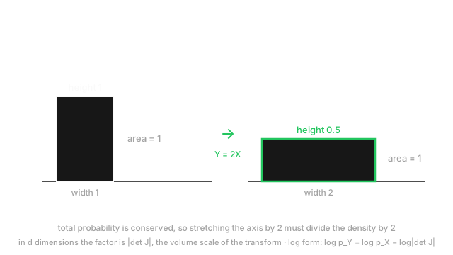
p_Y(y)\, |dy| = p_X(x)\, |dx| \quad \Longrightarrow \quad p_Y(y) = p_X(x) \left|\frac{dx}{dy}\right|

In plain words: the same probability mass now occupies an interval of a different width, so the height has to compensate. Stretch by a factor of 2 and $|dx/dy| = 1/2$ .

In several dimensions the derivative becomes a determinant

For $\mathbf{y} = g(\mathbf{x})$ with both in $\mathbb{R}^d$ , the local stretch is described by the Jacobian matrix $J_g$ , whose $(i,j)$ entry is $\partial y_i / \partial x_j$ . The factor by which it scales volume is $|\det J_g|$ :

p_Y(\mathbf{y}) = p_X\big(g^{-1}(\mathbf{y})\big) \, \big| \det J_{g^{-1}}(\mathbf{y}) \big| = \frac{p_X(\mathbf{x})}{\big| \det J_{g}(\mathbf{x}) \big|}

In plain words: divide by how much the forward transform expanded volume. The two forms are equivalent because the Jacobian of an inverse is the inverse of the Jacobian, so their determinants are reciprocals.

In practice you always work with logs, because a product of $L$ determinants across $L$ flow layers underflows and because losses are log-densities anyway:

\log p_Y(\mathbf{y}) = \log p_X(\mathbf{x}) - \log \big| \det J_{g}(\mathbf{x}) \big|

This single line is the entire likelihood of a normalising flow. Push the data back through the inverse transforms to a Gaussian, evaluate the Gaussian's log-density, subtract a log-determinant per layer. Nothing else.

Why flow architectures look the way they do

A general $d \times d$ determinant costs $O(d^3)$ , which is unusable when $d$ is the dimension of an image. Every flow design is a way of making the determinant cheap, and once you know that, the architectures stop looking arbitrary:

Triangular Jacobians. If each output depends only on inputs at or before its own index, the Jacobian is triangular and its determinant is the product of the diagonal — $O(d)$ . This is exactly what autoregressive flows (MAF, IAF) enforce.
Coupling layers. Split the input in half, pass one half through unchanged, and use it to compute a scale and shift for the other half. The Jacobian is block-triangular, the determinant is the product of the scales, and the transform is trivially invertible. This is RealNVP and Glow, and it is the design most flows still use.
Permutations between layers. Necessary because a coupling layer leaves half its input untouched, and a permutation is free: its determinant is $\pm 1$ , so the log-determinant is 0.
Residual and continuous flows. Neural ODEs replace the determinant with a trace, which can be estimated cheaply. Different route to the same problem.

Two special cases you use constantly

Inverse transform sampling. Take $U \sim \mathrm{Uniform}(0,1)$ and set $Y = F^{-1}(U)$ for any CDF $F$ . Then $Y$ has density $p$ . The change-of-variables factor is $|dF^{-1}/du| = 1/p(y)$ by the CDF–PDF relationship, and multiplying by the uniform density of 1 gives back exactly $p(y)$ . This is how every non-Gaussian sampler in every library is built.

Affine transforms. For $Y = aX + b$ , the Jacobian is the constant $a$ , so $p_Y(y) = p_X((y-b)/a) / |a|$ . Every standardisation step you have ever applied does this, and the $1/|a|$ is why the log-likelihood of your model changes when you rescale your features.

Worked example

Start with the simplest case, where the answer is checkable without any calculus. Let $X \sim \mathrm{Uniform}(0,1)$ , so $p_X(x) = 1$ on $[0,1]$ . Let $Y = 2X$ .

$Y$ lives on $[0,2]$ . Its inverse is $x = y/2$ , so $|dx/dy| = 1/2$ , giving

p_Y(y) = p_X(y/2) \times \tfrac{1}{2} = 1 \times \tfrac{1}{2} = 0.5 \quad \text{on } [0,2]

In plain words: doubling the variable halved the density. Check the area: width 2 times height 0.5 is 1. The distribution did not become "less likely"; it spread over twice the range.

Now a non-linear transform, and the one that generates exponential samples. Let $X \sim \mathrm{Uniform}(0,1)$ again and set $Y = -\ln(X) / \lambda$ . Inverting, $x = e^{-\lambda y}$ , and

\left|\frac{dx}{dy}\right| = \lambda e^{-\lambda y} \quad \Longrightarrow \quad p_Y(y) = 1 \times \lambda e^{-\lambda y}

That is the exponential density with rate $\lambda$ , exactly. A uniform generator plus a logarithm produces exponential samples, and the change-of-variables factor is the density — nothing was fitted or approximated.

Now two dimensions, where the determinant earns its place. Take $X$ uniform on the unit square, so $p_X = 1$ on an area of 1. Apply the linear map

A = \begin{bmatrix} 2 & 1 \\ 0 & 1 \end{bmatrix}, \qquad \det A = 2

This is the same shear used in linear transformations: the unit square becomes a parallelogram of area 2. So

p_Y(\mathbf{y}) = \frac{p_X(\mathbf{x})}{|\det A|} = \frac{1}{2} = 0.5

In plain words: the region doubled in area, so the density halved. Area 2 times density 0.5 is 1, as it must be. The log-determinant term is $\log 2 = 0.693$ , and this is precisely the number a flow layer would subtract.

Finally, the case that catches people out in reporting. Suppose a model assigns a log-density of $-2.30$ to a data point measured in metres, and you switch to centimetres, so $Y = 100X$ per dimension. In $d$ dimensions the log-density changes by $-d \log 100$ :

\log p_Y = -2.30 - d \log 100 = -2.30 - 4.605\,d

For $d = 3$ that is $-16.12$ instead of $-2.30$ . The model is identical, the data is identical, and the reported number moved by 13.82 nats purely because of a unit change. Anyone comparing log-likelihoods or bits-per-dimension across differently preprocessed pipelines is comparing preprocessing.

Show Me the Code

1import numpy as np2
3rng = np.random.default_rng(0)4u = rng.uniform(size=200_000)                      # X ~ Uniform(0,1), shape (200000,)5
6y = 2 * u                                          # doubling halves the density7print(round(float(np.histogram(y, bins=20, range=(0, 2), density=True)[0].mean()), 3))8
9lam = 1.5                                          # inverse transform sampling10exp_samples = -np.log(u) / lam                     # should be Exponential(1.5)11print(round(float(exp_samples.mean()), 4), round(1 / lam, 4))   # -> 0.6676 0.666712
13A = np.array([[2.0, 1.0], [0.0, 1.0]])             # (2, 2) shear14print(float(np.linalg.det(A)), round(float(np.log(2.0)), 4))    # -> 2.0 0.693115
16box = rng.uniform(size=(400_000, 2)) * [3.0, 1.0]  # bounding box of area 317pre = box @ np.linalg.inv(A).T                     # map each point back to x-space18inside = float(np.mean((pre >= 0).all(1) & (pre <= 1).all(1)))19print(round(inside * 3, 3))                        # -> 1.996  measured area == |det A|20print(round(-2.30 - 3 * np.log(100), 2))           # -> -16.12  metres to centimetres

The exponential mean lands on $1/\lambda$ to three decimals — 0.6676 against 0.6667, within its own Monte Carlo error — so the transform is producing the exact density rather than an approximation. The doubled uniform averages 0.5 exactly. The area measurement recovers $|\det A| = 2$ without ever calling det, which is what "the determinant is the volume scale factor" means operationally. And the last line is the reporting hazard as a number: same model, same data, 13.82 nats apart.

Watch Out For

Comparing log-likelihoods or bits-per-dimension across different preprocessing

A density has units of "probability per unit volume", so its value depends on what a unit is. Change the units and every log-density shifts by the log-determinant of the rescaling — a constant that has nothing to do with model quality.

The concrete cases in generative modelling:

Pixel scaling. A model trained on $[0,1]$ pixels and one trained on $[0,255]$ differ in log-likelihood by $d \log 256 = 5.545 d$ nats. For a $32 \times 32 \times 3$ image that is 17,035 nats, which utterly dominates any real difference between the models.
Dequantisation. Image data is discrete, and a continuous density model assigns infinite likelihood to a discrete point mass unless noise is added. How much noise, and whether it is uniform or variational, changes the reported number. Published bits-per-dimension figures are only comparable when the dequantisation matches.
Any invertible preprocessing at all. A logit transform, a per-channel standardisation, a whitening matrix. Each contributes a log-determinant. Some papers report it, some fold it in, some omit it.

Bits-per-dimension exists to make numbers comparable across image sizes — it divides by $d$ and converts to base 2 — and it does not fix the units problem. The convention it assumes is $[0, 256)$ pixel values with uniform dequantisation, and a number computed under any other convention is not on the same scale despite carrying the same name.

What to do:

State the preprocessing whenever you report a likelihood. Data range, dequantisation scheme, and any transform's log-determinant.
Only compare models you evaluated yourself, under one pipeline. Reproduce a baseline rather than quoting its number.
Remember a continuous log-likelihood can be positive, since a density above 1 has a positive log. That is not a bug and not a probability above 1.
For ranking or optimisation, none of this matters — a constant offset has no gradient. It matters the moment you compare across pipelines.

Assuming a transform is invertible when it is not, or when its Jacobian is numerically singular

The formula requires a bijection with a non-vanishing determinant. Break either condition and you get a silently wrong likelihood rather than an error.

Non-invertible transforms. $Y = X^2$ maps both $+2$ and $-2$ to 4, so the density at 4 is the sum of two contributions and the single-branch formula undercounts by half. A ReLU is not invertible at all — it discards the sign of everything negative — which is why no flow uses one. tanh is invertible in principle and saturates in practice: at $|x| > 4$ its derivative is under $10^{-3}$ , so the log-determinant term becomes a large negative number driven by floating-point noise rather than by the data.

Determinants that vanish or explode. In a coupling layer the log-determinant is $\sum_i s_i$ , the sum of the log-scales. Nothing constrains those scales, and if the network outputs a scale near zero the transform is locally collapsing dimensions — the inverse is numerically undefined and the log-determinant runs to $-\infty$ . The likelihood improves as this happens, so the optimiser drives straight toward it. The training curve looks excellent right up to the nan.

The standard defences, all of which appear in production flow implementations:

Parameterise the log-scale, not the scale, and pass it through a bounded function. s = tanh(raw) * limit or s = log_sigmoid(raw) + c keeps the scale in a safe band by construction.
Constrain the transform to be monotone by construction. Spline flows enforce monotonicity per bin, which guarantees invertibility rather than hoping for it.
Assert the round trip in a test. assert np.allclose(inverse(forward(x)), x) catches a broken invertibility claim immediately, and it is a one-line test that most flow bugs fail.
Log the mean log-determinant per layer during training. A layer drifting toward large negative values is the early warning, visible long before the loss goes non-finite.
Check the determinant's sign, not just its magnitude. A sign flip mid-training means the transform passed through a singular point, and everything after it is suspect.

The Quick Version

Transform a random variable and its density is rescaled by the reciprocal of the local stretch factor, because total probability is conserved.
One dimension: $p_Y(y) = p_X(x)\,|dx/dy|$ . Several dimensions: divide by $|\det J_g|$ , because volume rather than length is what scales.
In log form, $\log p_Y = \log p_X - \log|\det J_g|$ . That single line is the entire likelihood of a normalising flow.
Flow architectures exist to make the determinant cheap: triangular Jacobians cost $O(d)$ , coupling layers give a product of scales, permutations contribute zero.
Inverse transform sampling is this formula. So is every affine standardisation you apply.
Densities are not invariant under reparameterisation. Rescaling pixels from $[0,1]$ to $[0,255]$ shifts a log-likelihood by $5.545d$ nats with no change to the model.
Bits-per-dimension does not fix that. Only compare likelihoods under one preprocessing pipeline, ideally one you ran yourself.
The transform must be invertible with a non-vanishing determinant. ReLU is out; saturating tanh and unbounded coupling scales are numerical traps.
Test the round trip and log the per-layer log-determinant. Both failures show up there before they show up as nan.