Math

Convexity and Loss Landscapes

Some surfaces have exactly one bottom and walking downhill always finds it; neural network surfaces do not, and the reason training still works is not what most people assume.

A zero gradient does not mean you have arrived: this curve has a flat spot that is not a minimum and a genuine minimum elsewhere, and only curvature tells the two apart

Why Does This Exist?

Two facts sit awkwardly together. Neural network loss surfaces are non-convex, which in classical optimisation means you have no guarantee of finding the best answer. And yet training works, reliably, at enormous scale.

The folk explanation is that gradient descent gets stuck in bad local minima and we tolerate it. That explanation is wrong, and the correct one is more useful: in high dimensions local minima are vanishingly rare, and what actually slows training down is saddle points and plateaus. Those have different symptoms and different fixes, so the distinction changes what you do when a run stalls.

This page also explains why classical ML feels different from deep learning. Linear regression, logistic regression and SVMs are convex, so they converge to the same answer every time regardless of seed. Neural networks are not, which is why reporting a single run is weak evidence and why seed variance is a real experimental concern.

Think of It Like This

Two landscapes, and the difference a dimension makes

Imagine being dropped blindfolded on a landscape and told to walk downhill.

On a smooth bowl, you will reach the bottom. There is one, every direction from it goes up, and your starting point is irrelevant. This is convex, and it is why convex problems are considered solved.

On a mountain range, where you end up depends entirely on where you started. Some valleys are deeper than others. This is the picture people carry for neural networks, and it is misleading — because the analogy is in two dimensions and the real problem has millions.

Here is what changes with dimension. To be trapped in a valley, the ground must rise in every direction you could walk. In two dimensions there are few directions and being trapped is easy. In a million dimensions there are a million directions, and needing all of them to rise is an extraordinary coincidence. Almost every flat spot has some direction that still goes down.

So you are rarely trapped. You are frequently on a mountain pass — flat underfoot, with a way down that takes a while to find. That is a saddle, and it explains a plateau rather than a permanent stop.

How It Actually Works

A function is convex when the straight line between any two points on its graph never dips below the graph:

f(\lambda x + (1-\lambda)y) \le \lambda f(x) + (1-\lambda) f(y) \quad \text{for } \lambda \in [0,1]

In plain words: chords lie above the surface. Bowl-shaped, no bumps.

For a twice-differentiable function the test is curvature: $f$ is convex exactly when its Hessian is positive semi-definite everywhere. Every direction curves upward or is flat, nowhere downward.

The payoff is a guarantee: any local minimum of a convex function is a global minimum. Walking downhill cannot mislead you, convergence is provable, and the result does not depend on initialisation.

What breaks convexity

Convexity is fragile, and neural networks break it immediately. Composing convex functions does not preserve convexity — ReLU is convex and a linear map is convex, but stacking them is not. Even without nonlinearity, permutation symmetry alone destroys uniqueness: swap two hidden neurons along with their weights and the loss is identical, so a network with $k$ neurons in a layer has at least $k!$ equivalent minima.

What remains convex: linear and ridge regression, logistic regression, SVMs, lasso, and any linear model with a convex loss. That is a large and useful part of classical ML, and it is why those models are reproducible.

Classifying a flat spot

At a point where the gradient is zero, the Hessian's eigenvalue signs decide what you found:

All positive — a local minimum. Every direction curves up.
All negative — a local maximum.
Mixed — a saddle. Some directions up, some down.
Some zero — a plateau or a flat valley floor; the second-order test is inconclusive.

The counting argument

Here is the argument that overturns the folk story. For a stationary point to be a minimum, every eigenvalue must be positive. Treat the signs as roughly independent coin flips — a crude model, but the conclusion is robust — and the probability that all $n$ are positive is about $2^{-n}$ .

At $n = 10$ that is 1 in 1,024. At $n = 1000$ it is $10^{-301}$ . In a network with millions of parameters, essentially every stationary point is a saddle.

This has been checked empirically, and the finding is stronger still: the local minima that do exist in large networks tend to have similar loss values. So the classical worry — getting stuck somewhere much worse than the global optimum — is largely not what happens. Saddles and plateaus slow you down; they do not trap you, because a descent direction exists.

What that means in practice

Momentum helps because it carries velocity through regions where the gradient is nearly zero, escaping plateaus that would stall plain gradient descent.
Stochastic gradients help because minibatch noise perturbs you off a saddle. Noise is a feature here.
A plateau is not convergence. Watch the gradient norm: near a saddle it is small but the Hessian still has negative eigenvalues, so there is progress available.
Seeds matter. Different initialisations reach different minima, so a single run is a single sample. Report mean and spread across seeds.
Flat minima are believed to generalise better than sharp ones, since a wide basin is less sensitive to the shift between training and test distributions. This motivates sharpness-aware minimisation, and it remains an active area rather than settled fact.

Worked example

Take $f(x) = x^4 - 3x^3 + 2$ , and find its flat spots.

f'(x) = 4x^3 - 9x^2 = x^2(4x - 9)

Setting this to zero gives $x = 0$ and $x = 9/4 = 2.25$ . Two stationary points. Now the curvature:

f''(x) = 12x^2 - 18x

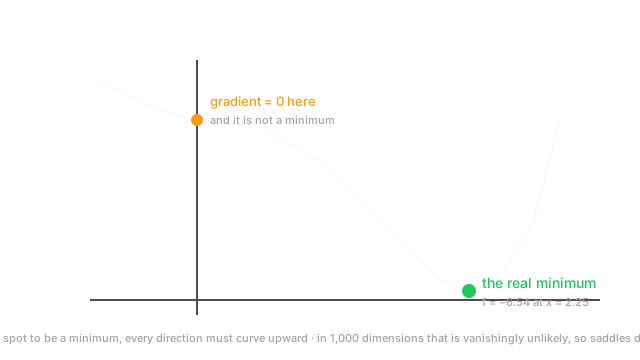
At $x = 0$ : $f''(0) = 0$ . Inconclusive — and in fact this is not a minimum. Check the neighbours: $f(-0.1) \approx 2.003$ and $f(0.1) \approx 1.997$ , so the function is decreasing through $x = 0$ . It is a flat inflection point, with $f(0) = 2$ .

At $x = 2.25$ : $f''(2.25) = 12(5.0625) - 40.5 = 60.75 - 40.5 = 20.25 > 0$ . A genuine minimum, and

f(2.25) = 25.6289 - 34.1719 + 2 = -6.543

So a zero gradient occurred at a point that is 8.5 units worse than the actual minimum, and the gradient alone could not tell the difference. Only $f''$ resolved it.

Gradient descent started anywhere below 2.25 moves right, since $f' < 0$ there — except at exactly $x = 0$ , where the gradient is exactly zero and plain gradient descent would stop forever. Momentum would carry through it. That is the plateau problem in one dimension, and the diagram shows both points.

Show Me the Code

1import numpy as np2
3f = lambda x: x**4 - 3 * x**3 + 24f1 = lambda x: 4 * x**3 - 9 * x**25f2 = lambda x: 12 * x**2 - 18 * x6
7for x in (0.0, 2.25):8    print(x, round(f(x), 4), round(f1(x), 6), round(f2(x), 4))9# -> 0.0 2.0 0.0 0.0        gradient zero, curvature zero: NOT a minimum10# -> 2.25 -6.543 0.0 20.25  gradient zero, curvature positive: a minimum11
12# Plain gradient descent started exactly on the plateau never leaves.13x, lr = 0.0, 0.0114for _ in range(500):15    x -= lr * f1(x)16print(round(x, 6))                                  # -> 0.0  stuck17
18# Momentum carries through it.19x, v, beta = 0.0, 0.0, 0.920for _ in range(500):21    v = beta * v - lr * f1(x)22    x += v23print(round(x, 4))                                  # -> 2.25  escaped, found the min24
25# The counting argument: P(all n eigenvalues positive) ~ 2^-n.26for n in (1, 10, 100):27    print(n, f"{2.0 ** -n:.3e}")     # -> 1 5.000e-01 | 10 9.766e-04 | 100 7.889e-31

The two stationary points and their curvatures match the hand calculation, and the two descent loops demonstrate the plateau: identical starting point, and only momentum reaches $-6.543$ .

Watch Out For

Diagnosing a plateau as convergence

A small gradient norm looks like convergence and usually is not. Near a saddle the gradient is genuinely tiny while the loss is nowhere near a minimum, and there is a descent direction available that first-order information cannot see.

The practical consequence is stopping too early. An early-stopping rule keyed on "loss stopped improving for $k$ steps" fires on a plateau, and you ship a model that had substantial progress remaining. Long plateaus followed by sharp drops are a well-documented pattern in deep learning, and any patience shorter than the plateau discards the drop.

Distinguishing the two cases needs curvature, not the gradient. If the Hessian has a negative eigenvalue you are at a saddle; if all are positive you are at a minimum. You can test this cheaply without building the Hessian — power iteration on Hessian-vector products estimates the extreme eigenvalues in a handful of gradient-cost operations.

The cheaper habits usually suffice. Log the gradient norm alongside the loss, since a norm that is small but not collapsing is a plateau signature. Use momentum and minibatch noise, both of which escape saddles by construction. And set early-stopping patience generously, measured against how long plateaus actually last in your setup rather than a default.

Reporting one run of a non-convex optimisation

Because the surface is non-convex, the result depends on initialisation, data ordering, and every source of randomness. One run is one sample from a distribution of outcomes, and the spread is often larger than the improvements people report.

The failure is systematic rather than random. You try a change, run once, see a better number, and keep it — which is selection on noise. Repeat that a dozen times over a project and you have accumulated a model that looks better on your validation set and is not, exactly the multiple comparisons problem wearing a different hat.

Seed variance in deep learning routinely reaches one or two points of accuracy, which is the same size as most claimed improvements. So a single-run comparison of two architectures is not evidence about the architectures.

Three habits. Run at least three seeds and report mean with standard deviation; if the change is smaller than the seed spread, you have not measured it. Fix and record every seed — framework, NumPy, Python, dataloader workers — because reproducibility is a prerequisite for the rest. And compare distributions rather than maxima: reporting the best of five seeds against a baseline's single run is the dart-throwing problem, and it inflates results reliably.

The Quick Version

Convex means chords lie above the surface, equivalently the Hessian is positive semi-definite everywhere.
Any local minimum of a convex function is global. That is the whole value of convexity.
Linear and ridge regression, logistic regression, lasso and SVMs are convex. Neural networks are not.
Composing convex functions does not preserve convexity, and permutation symmetry alone gives $k!$ equivalent minima per layer.
At a zero gradient, Hessian signs decide: all positive is a minimum, mixed is a saddle, some zero is inconclusive.
Saddles dominate in high dimensions, because a minimum needs every eigenvalue positive — roughly $2^{-n}$ .
The classical fear of bad local minima is largely not what happens; large-network minima tend to have similar loss.
Plateaus and saddles slow training rather than stopping it. Momentum and minibatch noise escape them.
A small gradient norm is not convergence. Log it alongside the loss and set patience generously.
Flat minima are believed to generalise better than sharp ones — motivation for sharpness-aware methods, not settled fact.
Non-convexity means seeds matter. Run three or more and report the spread.