Data Concepts

Noise, Outliers and Anomaly Detection

The same statistics, the opposite action. A height of 3.2 metres is a typing mistake you delete; an odd transaction is the fraud you were hired to catch.

A row can sit inside the normal range on every axis on its own and still be far outside the cloud those axes form together, which is exactly the outlier a column-by-column screen never sees

Why Does This Exist?

Two rows in a hospital dataset. One records a patient height of 3.2 metres. One records a heart rate of 210 in a resting adult.

Both sit far out in the tail. Both get flagged by any threshold you write. And the correct handling is opposite: the height is a decimal point in the wrong place and should go, while the heart rate may be the event the whole model exists to predict. Delete the second and you've removed your positive class.

Detection tells you a value is unusual. It cannot tell you whether unusual means broken. Fraud, equipment failure, disease onset, network intrusion, a market shock — every one is an outlier you must keep, and some are the label. So the first question is about provenance, not statistics: could this measurement physically have happened?

Three words that get used interchangeably and shouldn't. Noise is small random error around a true value, in every measurement, and you model through it. An outlier is a point far from the rest, error or real. An anomaly is a point you want to find, because finding it is the job.

Think of It Like This

A flatline on a hospital monitor

A bedside monitor goes flat and the alarm sounds. Two things produce that trace, and they're as far apart as two things get.

An electrode came unstuck. The patient is fine, sitting up, mildly annoyed by the noise, and the fix is to reattach the lead. Or the heart has stopped, the reading is accurate, and every second spent doubting the equipment is a second lost.

The trace is identical. Nurses are trained for exactly this: look at the patient, not the machine. What separates the two cases is never in the signal — it's in the world the signal came from.

That's your outlier. The statistic tells you the value is extreme. Whether it's a loose lead or a cardiac arrest comes from knowing how the number was produced.

How It Actually Works

Detection splits along one axis that matters more than the choice of algorithm: are you looking at one column at a time, or at the row as a whole?

One column at a time

The z-score, and the 3-sigma rule on top of it, measures distance from the mean in standard deviations and flags anything past three. Tukey's IQR rule flags anything outside $[Q_1 - 1.5 \cdot \text{IQR},\; Q_3 + 1.5 \cdot \text{IQR}]$ , where $Q_1$ and $Q_3$ are the 25th and 75th percentiles and IQR is the gap between them. The modified z-score swaps in order statistics throughout:

z = \frac{x - \bar{x}}{s} \qquad\text{versus}\qquad z_{\text{mod}} = \frac{0.6745\,(x - \tilde{x})}{\text{MAD}}

On the left, $\bar{x}$ is the mean and $s$ the standard deviation. On the right, $\tilde{x}$ is the median and MAD is the median absolute deviation — the median of how far each point sits from the median. The 0.6745 makes the two scores agree on normal data, so the usual cutoff is around 3.5.

The left-hand version has a defect its popularity hides. Both the mean and the standard deviation are computed including the outlier, and a large outlier inflates both, so it widens the very threshold it's tested against and past a certain size it hides itself. That's called masking, and with a handful of extreme values a 3-sigma screen can return nothing at all.

The IQR rule and the modified z-score are built from percentiles, and a percentile moves by at most one position no matter how extreme a single value gets. That's what "robust to outliers" means, and why these two are the defaults while 3-sigma is reserved for data you already know is roughly normal. Descriptive statistics has the full sensitivity comparison.

The whole row at once

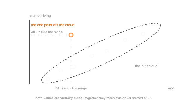
A row can be unremarkable in every column and impossible in combination. A 3-year-old with a driving licence. The diagram above shows it with numbers: age 34 is ordinary, 40 years behind the wheel is ordinary, and together they describe someone who started driving at minus six. No column-by-column screen sees that, because no column holds anything strange.

Four methods that do:

Mahalanobis distance measures distance from the data's centre after accounting for how the columns co-vary, so "far" stretches along the directions the data actually spreads in. Assumes one elliptical cloud, which real data often isn't.
Isolation forest splits the data with random cuts and counts how few it takes to isolate each point. Odd points fall out early. Fast, scales well, handles many columns, and the usual first reach.
Local outlier factor compares a point's local density with its neighbours', so it catches a point that's odd relative to its own cluster when the data has several clusters at different densities.
One-class SVM learns a boundary around the normal region. Sensitive to its kernel settings and to how much contamination you assume.

All four use distance, so all four need scaled columns first. Run isolation forest on raw income and raw age and income decides everything.

What to do about it, in order

Deleting is last, not first.

Investigate. Pull the raw record. Ten minutes here often turns up a unit change or a broken sensor, and fixes a whole class of rows rather than one.
Fix it when the true value is recoverable — a misplaced decimal, kilograms recorded as grams, a timezone.
Cap it. Winsorising pulls extremes back to a percentile, usually the 1st and 99th. Keeps the row and the direction, drops the magnitude.
Transform it. A log or a Box-Cox compresses a long right tail so extremes stop dominating, without discarding anything. See non-linear transformations.
Change the model. Trees barely notice extreme feature values, since a split only cares about order. For linear models, a Huber loss is quadratic near zero and linear in the tails, so one bad point pulls the fit far less than squared error does.
Drop it, with the reason recorded. Fine when you can name the cause. Not fine as a way to move a metric.

Worked example

Ten values: 10, 11, 12, 12, 13, 13, 14, 14, 15, 66.

They sum to 180, so the mean is 18.0. The standard deviation is 16.062, most of it contributed by the 66 alone. The 3-sigma ceiling is therefore

18.0 + 3 \times 16.062 = 66.187

and the value under test is 66. Nothing gets flagged. Its z-score is 2.99, just under the line, because the point pushed the line out past itself.

Now the percentile route. Sorted, the 25th percentile is 12 and the 75th is 14, so the IQR is 2 and the upper fence is $14 + 1.5 \times 2 = 17$ . The 66 clears that by nearly four times.

The modified z-score is starker. The median is 13, the absolute deviations are mostly 0, 1 or 2, and their median — the MAD — is 1, giving $0.6745 \times (66 - 13) / 1 = 35.7$ against a cutoff of 3.5.

Same ten numbers. One rule says 2.99 and shrugs; the other says 35.7.

Show Me the Code

1import numpy as np2
3x = np.array([10, 11, 12, 12, 13, 13, 14, 14, 15, 66], dtype=float)4med = float(np.median(x))5
6
7def iqr_upper(v: np.ndarray) -> float:8    """Percentile-built, so one extreme value barely moves the fence."""9    q1, q3 = np.percentile(v, [25, 75])10    return float(q3 + 1.5 * (q3 - q1))11
12
13mad = float(np.median(np.abs(x - med)))           # median absolute deviation14
15print(x.mean(), round(x.std(), 3))                # -> 18.0 16.06216print(round(x.mean() + 3 * x.std(), 3), x.max())  # -> 66.187 66.0  nothing flagged17print(iqr_upper(x))                               # -> 17.0        66 clears this fence18print(med, mad)                                   # -> 13.0 1.019print(round(0.6745 * (x.max() - med) / mad, 1))   # -> 35.7        the robust score

The gap between 66.187 and 17.0 is the entire argument for percentile-based rules.

Watch Out For

Dropping outliers because the metric improves

RMSE falls, the residual plot tidies up, and it feels like cleaning. Check what left.

On a claims model, the expensive claims are the tail. On a churn model, the heavy users. On a demand forecast, the spike you were asked to plan capacity for. Removing them makes the model excellent at the middle of the distribution, which is the part nobody needed a model for, and the error you get charged for lives in the part you deleted.

A quieter second effect: a StandardScaler refitted on the trimmed column has a smaller standard deviation, so in production, where the tail arrives whether you like it or not, those rows scale to values the model never saw. You didn't remove the tail. You removed your ability to handle it.

Two questions before any deletion. Can I name a physical cause? Is the tail part of what I'm graded on? Two noes means cap, transform, or change the loss.

Screening every column independently and calling it cleaning

for col in df.columns: df = df[iqr_mask(df[col])]. It looks thorough. It's a row shredder.

Each column removes its own small percentage, and the survivors are the intersection. With 20 columns and a rule flagging roughly 1% per column, the fraction surviving all 20 is $0.99^{20} = 0.818$ , so you lose about 18% of your data — to nothing in particular, since almost every deleted row was flagged by one column and fine in the other 19. On a table with 100 columns you'd keep 37% of your rows.

The deletion isn't neutral either. Rows extreme on one dimension are likelier to be extreme on a correlated one, so you're removing a structured slice rather than a random sample. Same population shift missing data warns about, through a different door.

Score the row, not the columns. One isolation forest or one Mahalanobis distance over scaled columns gives a single number per row you can rank, inspect and threshold once — and you get to look at the top 50 before deciding anything.

The Quick Version

Ask whether the value is a broken measurement or the rare event you're paid to catch. Detection can't answer that; provenance can.
Noise is random error you model through. An outlier is far from the rest. An anomaly is the thing you're hunting.
3-sigma uses the mean and standard deviation the outlier itself inflated, so large outliers mask themselves. The IQR rule and the modified z-score come from percentiles and don't.
On ten values ending in 66, the 3-sigma ceiling is 66.187 and flags nothing. The IQR fence is 17.0, the robust score 35.7.
A row can be ordinary in every column and impossible in combination. Age 34 with 40 years of driving.
For whole-row detection: Mahalanobis, isolation forest, local outlier factor, one-class SVM. All need scaled columns.
Actions in order: investigate, fix, cap, transform, change the model or loss, then drop with a recorded reason.
Deleting to move a metric removes the tail you're graded on, and quietly refits every scaler downstream.
Column-by-column filtering compounds: 20 columns at 1% each costs 18% of your rows. Score rows instead.