Monte Carlo Methods

Why Does This Exist?

Because grid-based integration dies in high dimensions and machine learning lives there.

Slice each axis into 10 pieces and a $d$-dimensional integral needs $10^d$ evaluations. In 3 dimensions that is 1,000 and fine. In 100 dimensions it is $10^{100}$, which exceeds the number of atoms in the observable universe. Every deterministic quadrature rule has this exponent, and a latent space, a parameter vector or a token distribution has hundreds to billions of dimensions.

Monte Carlo estimation has an error that scales as $1/\sqrt{n}$ with no $d$ in it at all. The dimension affects how large the constant is, but not the exponent. That single property is why sampling, rather than integration, is how modern machine learning computes expectations, and it is not an approximation people settle for — it is the only thing that works.

Five things you use are Monte Carlo estimates, and it is worth recognising them as the same operation:

• Every minibatch gradient. The true gradient is an average over the whole dataset; a batch of 32 is a Monte Carlo estimate of it. This is why gradient noise scales as $1/\sqrt{\text{batch size}}$ and why quadrupling the batch halves the noise rather than quartering it.
• Every sampled generation. Temperature sampling, top-$k$, nucleus sampling — drawing a token from a distribution rather than taking the argmax.
• The reparameterisation trick in a VAE. The expectation in the ELBO is estimated with a single sample per datapoint. One sample is a terrible estimator with enormous variance, and it works because SGD averages over batches and steps.
• Dropout at inference time (MC dropout). Run the network 30 times with dropout left on and average. That is a Monte Carlo estimate of a predictive distribution.
• Bootstrap resampling. Resampling your data to get an interval on a statistic is Monte Carlo applied to the empirical distribution.

Think of It Like This

How It Actually Works

Any integral can be written as an expectation, and any expectation can be estimated by an average. That is the entire method in two steps.

Given a distribution $p(x)$ and a function $f$:

In plain words: draw $n$ samples from $p$, apply $f$ to each, average. If your integral has no $p$ in it, insert one — $\int_a^b g(x)\, dx = (b-a)\,\mathbb{E}_{U(a,b)}[g(X)]$ turns any definite integral into an expectation over the uniform distribution.

Two guarantees make this legitimate rather than merely plausible.

It is unbiased. $\mathbb{E}[\hat{\mu}_n] = \mathbb{E}_p[f(X)]$ for every $n$, including $n = 1$. The estimator is centred on the right answer immediately; more samples reduce its spread, not a systematic offset. This is why a one-sample ELBO estimate is not wrong, merely noisy.

Its error is quantified. By the central limit theorem, $\hat{\mu}_n$ is approximately Gaussian around the true value with standard deviation

In plain words: the spread of your estimate is the spread of $f$ divided by the square root of the sample count. You can compute this from the same samples, using their observed standard deviation — so a Monte Carlo estimate always comes with an error bar, for free, and quoting one without it is throwing away half the output.

Reading the $1/\sqrt{n}$ law honestly

Two consequences, and they point in opposite directions.

It is slow. One extra decimal digit costs $100\times$ the samples. Three digits of precision from a plain Monte Carlo estimate is a serious computation, which is why sampling is never the answer for a low-dimensional integral where quadrature converges far faster.

It is dimension-free. Grid quadrature costs $O(k^d)$. Monte Carlo costs $O(n)$ for a fixed relative error regardless of $d$. There is a crossover, and it arrives early — around 4 to 6 dimensions for smooth functions. Above that, sampling is not just better, it is the only option.

The variance $\sigma^2$ does depend on the problem, and reducing it is where all the engineering is. Three levers, in the order they are usually reached for:

• Importance sampling. Sample from a different distribution $q$ that puts mass where $f$ is large, and reweight: $\mathbb{E}_p[f] = \mathbb{E}_q[f \cdot p/q]$. With a well-chosen $q$ the variance drops by orders of magnitude. With a badly chosen one it becomes infinite, which the second pitfall covers.
• Antithetic and common random numbers. Pair each sample with its mirror image so their errors cancel. Cheap, and it is why fixing the seed when comparing two configurations makes small differences measurable.
• Control variates. Subtract something correlated with $f$ whose expectation you already know. This is exactly what a baseline does in REINFORCE, and it is the difference between policy gradients that train and policy gradients that do not.

When you cannot sample directly

Everything above assumes you can draw from $p$. Often you cannot — a Bayesian posterior is known only up to its normalising constant, so you can evaluate $\tilde{p}(x) \propto p(x)$ but not sample from it.

Markov chain Monte Carlo solves this with a walk. Propose a move, accept it with a probability that depends only on the ratio $\tilde{p}(x') / \tilde{p}(x)$ — in which the unknown normaliser cancels — and the chain's long-run distribution is $p$. That cancellation is the whole trick, and it is why MCMC can sample a distribution nobody can normalise.

The cost is that consecutive samples are correlated, so $n$ draws carry less information than $n$ independent ones, and the chain needs time to forget where it started. In practice: discard a burn-in period, run several chains, and check convergence with $\hat{R}$ and effective sample size as described in Bayesian inference. Modern samplers — Hamiltonian Monte Carlo and NUTS — use the gradient of $\log \tilde{p}$ to propose better moves, which is the same gradient your autodiff system already computes.

Worked example

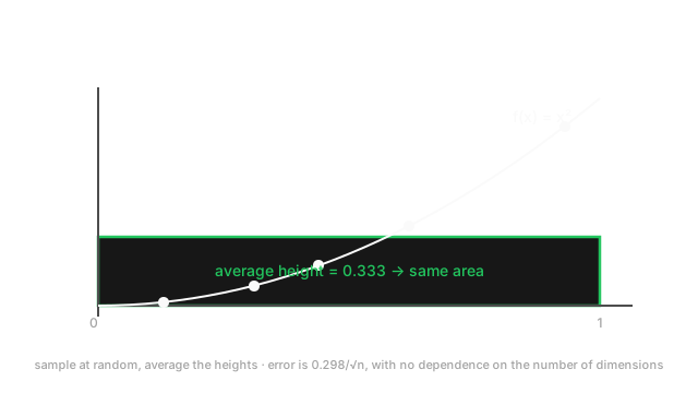
Estimate $\int_0^1 x^2\, dx$, whose exact value is $\tfrac{1}{3} = 0.3333$, by sampling. This is a case where Monte Carlo is the wrong tool — one dimension, closed form available — and that is exactly why it is the right example: you can check every number against the truth.

Write the integral as an expectation over the uniform distribution on $[0,1]$, where the density is 1:

Now the error bar, before running anything. The variance of $f(X) = X^2$ under $U(0,1)$ uses $\mathbb{E}[X^4] = \tfrac{1}{5}$ and $\mathbb{E}[X^2] = \tfrac{1}{3}$:

So $\sigma = 0.2981$, and the standard error at each sample size follows immediately:

In plain words: with 100 samples expect to be within about 0.03 of $\tfrac{1}{3}$; with 10,000, within about 0.003. A hundredfold increase in work for a tenfold improvement, predicted in advance, without running the estimator once.

Running it confirms both the estimates and the error bars, and the code below prints the observed errors alongside the predicted ones so you can see them agree.

Now the dimension-free claim, made concrete. Estimate $\mathbb{E}[\lVert X \rVert^2]$ for $X$ uniform on the unit cube in $d$ dimensions. Each coordinate contributes $\mathbb{E}[X_j^2] = \tfrac{1}{3}$, so the answer is $d/3$ exactly — 0.333 in 1 dimension, 33.33 in 100 dimensions. The relative standard error is what to watch: with 10,000 samples it is about 0.9% in one dimension and about 0.09% in a hundred. It got better, because summing 100 coordinates averages away their individual noise. Grid quadrature would need $10^{100}$ evaluations to attempt the same integral at all.

Show Me the Code

1import numpy as np2
3rng = np.random.default_rng(0)4TRUE, SIGMA = 1 / 3, np.sqrt(4 / 45)                 # exact answer and exact sd of x^25
6for n in (100, 10_000, 1_000_000):7    f = rng.uniform(size=n) ** 2                     # f(x) = x^2, shape (n,)8    est, se = float(f.mean()), float(f.std(ddof=1) / np.sqrt(n))9    print(n, round(est, 4), f"se={se:.4f}", f"predicted={SIGMA / np.sqrt(n):.4f}",10          f"error={abs(est - TRUE):.4f}")11# -> 100     0.3925 se=0.0324 predicted=0.0298 error=0.059212# -> 10000   0.3327 se=0.0030 predicted=0.0030 error=0.000713# -> 1000000 0.3336 se=0.0003 predicted=0.0003 error=0.000314
15# Dimension-free: the relative error IMPROVES with d, it does not degrade.16for d in (1, 100):17    f = (rng.uniform(size=(10_000, d)) ** 2).sum(axis=1)          # ||x||^2, shape (10000,)18    print(d, round(float(f.mean()), 3), f"true={d / 3:.3f}",19          f"rel_se={f.std(ddof=1) / np.sqrt(10_000) / f.mean():.5f}")20# -> 1   0.342  true=0.333  rel_se=0.0088021# -> 100 33.326 true=33.333 rel_se=0.00090

The observed standard errors match the predicted ones — 0.0324 against 0.0298, 0.0030 against 0.0030 — so the error bar is trustworthy even when computed from the same samples as the estimate.

The $n = 100$ row is worth sitting with. The estimate is 0.3925, off by 0.0592, which is about 1.8 standard errors. Nothing has gone wrong: a $\pm 1$ standard error band covers only 68% of the time, so a 1.8-sigma miss is entirely ordinary and will happen on roughly one seed in fourteen. That is precisely why the error bar has to be reported rather than the estimate alone. Anyone who ran only this seed and quoted 0.39 as the answer would be 18% high with no way to know.

The second loop is the property the method exists for: a hundredfold increase in dimension, the same 10,000 samples, and the relative error went down tenfold rather than up.

Watch Out For

The Quick Version

• Monte Carlo replaces an integral with an average over random samples: $\mathbb{E}_p[f] \approx \frac{1}{n}\sum f(x_i)$.
• The estimator is unbiased at every $n$, so a one-sample estimate is noisy rather than wrong.
• The standard error is $\sigma/\sqrt{n}$ and is computable from the same samples. A Monte Carlo number without an error bar is incomplete.
• $1/\sqrt{n}$ is slow: one more decimal digit costs a hundredfold more samples.
• $1/\sqrt{n}$ contains no $d$. That is the whole reason the method exists, and why grid quadrature is unusable above about 6 dimensions.
• Variance reduction is where the engineering is: importance sampling, antithetic variates, control variates. A REINFORCE baseline is a control variate.
• MCMC samples distributions known only up to a constant, because the accept ratio cancels the normaliser. The price is correlated samples and convergence diagnostics.
• Minibatch gradients, temperature sampling, the VAE reparameterisation trick, MC dropout and the bootstrap are all this same operation.
• Importance weights with a light-tailed proposal give infinite variance and a stable-looking wrong answer. Check effective sample size.

What to Read Next

• Integration and Area Under a Curve is the deterministic alternative, and where the curse of dimensionality that motivates sampling is laid out.
• Expectation, Variance and Covariance supplies the $\sigma^2$ in the error formula.
• Central Limit Theorem is what makes the error Gaussian and the error bar meaningful.
• Bayesian Inference is the main consumer, and where MCMC diagnostics live.
• Bootstrap and Resampling is Monte Carlo applied to your own dataset.
• Definitions worth a look: Expected Value, Variance, Standard Deviation, and Random Variable.
• Related interview question: Compute a variance in one pass